[深度应用]·Keras极简实现Attention结构

[深度应用]·Keras极简实现Attention结构

在上篇博客中笔者讲解来Attention结构的基本概念,在这篇博客使用Keras搭建一个基于Attention结构网络加深理解。。

1.生成数据 

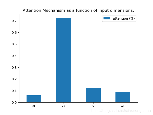
这里让x[:, attention_column] = y[:, 0],X数据的第一列等于Y数据第零列(其实就是label),这样第一列数据和label的相关度就会很大,最后通过输出相关度来证明思路正确性。

import keras.backend as K
import numpy as np


def get_activations(model, inputs, print_shape_only=False, layer_name=None): # Documentation is available online on Github at the address below. # From: https://github.com/philipperemy/keras-visualize-activations print('----- activations -----') activations = [] inp = model.input if layer_name is None: outputs = [layer.output for layer in model.layers] else: outputs = [layer.output for layer in model.layers if layer.name == layer_name] # all layer outputs funcs = [K.function([inp] + [K.learning_phase()], [out]) for out in outputs] # evaluation functions layer_outputs = [func([inputs, 1.])[0] for func in funcs] for layer_activations in layer_outputs: activations.append(layer_activations) if print_shape_only: print(layer_activations.shape) else: print(layer_activations) return activations def get_data(n, input_dim, attention_column=1): """ Data generation. x is purely random except that it's first value equals the target y. In practice, the network should learn that the target = x[attention_column]. Therefore, most of its attention should be focused on the value addressed by attention_column. :param n: the number of samples to retrieve. :param input_dim: the number of dimensions of each element in the series. :param attention_column: the column linked to the target. Everything else is purely random. :return: x: model inputs, y: model targets """ x = np.random.standard_normal(size=(n, input_dim)) y = np.random.randint(low=0, high=2, size=(n, 1)) x[:, attention_column] = y[:, 0] return x, y 

2.定义网络

import matplotlib.pyplot as plt
import pandas as pd
import numpy as np from attention_utils import get_activations, get_data np.random.seed(1337) # for reproducibility from keras.models import * from keras.layers import Input, Dense,Multiply,Activation input_dim = 4 def Att(att_dim,inputs,name): V = inputs QK = Dense(att_dim,bias=None)(inputs) QK = Activation("softmax",name=name)(QK) MV = Multiply()([V, QK]) return(MV) def build_model(): inputs = Input(shape=(input_dim,)) atts1 = Att(input_dim,inputs,"attention_vec") x = Dense(16)(atts1) atts2 = Att(16,x,"attention_vec1") output = Dense(1, activation='sigmoid')(atts2) model = Model(input=inputs, output=output) return model

3.训练与作图

if __name__ == '__main__':
    N = 10000
    inputs_1, outputs = get_data(N, input_dim)

    print(inputs_1[:2],outputs[:2]) m = build_model() m.compile(optimizer='adam', loss='binary_crossentropy', metrics=['accuracy']) print(m.summary()) m.fit(inputs_1, outputs, epochs=20, batch_size=128, validation_split=0.2) testing_inputs_1, testing_outputs = get_data(1, input_dim) # Attention vector corresponds to the second matrix. # The first one is the Inputs output. attention_vector = get_activations(m, testing_inputs_1, print_shape_only=True, layer_name='attention_vec')[0].flatten() print('attention =', attention_vector) # plot part. pd.DataFrame(attention_vector, columns=['attention (%)']).plot(kind='bar', title='Attention Mechanism as ' 'a function of input' ' dimensions.') plt.show()

4.结果展示

实验结果表明,第一列相关性最大,符合最初的思想。

__________________________________________________________________________________________________
Layer (type)                    Output Shape         Param #     Connected to                     
==================================================================================================
input_1 (InputLayer)            (None, 4)            0                                            
__________________________________________________________________________________________________
dense_1 (Dense)                 (None, 4) 16 input_1[0][0] __________________________________________________________________________________________________ attention_vec (Activation) (None, 4) 0 dense_1[0][0] __________________________________________________________________________________________________ multiply_1 (Multiply) (None, 4) 0 input_1[0][0] attention_vec[0][0] __________________________________________________________________________________________________ dense_2 (Dense) (None, 16) 80 multiply_1[0][0] __________________________________________________________________________________________________ dense_3 (Dense) (None, 16) 256 dense_2[0][0] __________________________________________________________________________________________________ attention_vec1 (Activation) (None, 16) 0 dense_3[0][0] __________________________________________________________________________________________________ multiply_2 (Multiply) (None, 16) 0 dense_2[0][0] attention_vec1[0][0] __________________________________________________________________________________________________ dense_4 (Dense) (None, 1) 17 multiply_2[0][0] ================================================================================================== Total params: 369 Trainable params: 369 Non-trainable params: 0 __________________________________________________________________________________________________ None Train on 8000 samples, validate on 2000 samples Epoch 1/20 2019-05-26 20:02:22.289119: I tensorflow/core/platform/cpu_feature_guard.cc:141] Your CPU supports instructions that this TensorFlow binary was not compiled to use: SSE4.1 SSE4.2 AVX AVX2 FMA 2019-05-26 20:02:22.290211: I tensorflow/core/common_runtime/process_util.cc:69] Creating new thread pool with default inter op setting: 4. Tune using inter_op_parallelism_threads for best performance. 8000/8000 [==============================] - 2s 188us/step - loss: 0.6918 - acc: 0.5938 - val_loss: 0.6893 - val_acc: 0.7715 Epoch 2/20 8000/8000 [==============================] - 0s 23us/step - loss: 0.6848 - acc: 0.7889 - val_loss: 0.6774 - val_acc: 0.8065 Epoch 3/20 8000/8000 [==============================] - 0s 28us/step - loss: 0.6619 - acc: 0.8091 - val_loss: 0.6417 - val_acc: 0.7780 Epoch 4/20 8000/8000 [==============================] - 0s 29us/step - loss: 0.6132 - acc: 0.8166 - val_loss: 0.5771 - val_acc: 0.8610 Epoch 5/20 8000/8000 [==============================] - 0s 28us/step - loss: 0.5304 - acc: 0.8925 - val_loss: 0.4758 - val_acc: 0.9185 Epoch 6/20 8000/8000 [==============================] - 0s 28us/step - loss: 0.4177 - acc: 0.9433 - val_loss: 0.3554 - val_acc: 0.9680 Epoch 7/20 8000/8000 [==============================] - 0s 24us/step - loss: 0.3028 - acc: 0.9824 - val_loss: 0.2533 - val_acc: 0.9930 Epoch 8/20 8000/8000 [==============================] - 0s 40us/step - loss: 0.2180 - acc: 0.9961 - val_loss: 0.1872 - val_acc: 0.9985 Epoch 9/20 8000/8000 [==============================] - 0s 37us/step - loss: 0.1634 - acc: 0.9986 - val_loss: 0.1442 - val_acc: 0.9985 Epoch 10/20 8000/8000 [==============================] - 0s 33us/step - loss: 0.1269 - acc: 0.9998 - val_loss: 0.1140 - val_acc: 0.9985 Epoch 11/20 8000/8000 [==============================] - 0s 22us/step - loss: 0.1013 - acc: 0.9998 - val_loss: 0.0921 - val_acc: 0.9990 Epoch 12/20 8000/8000 [==============================] - 0s 28us/step - loss: 0.0825 - acc: 0.9999 - val_loss: 0.0758 - val_acc: 0.9995 Epoch 13/20 8000/8000 [==============================] - 0s 22us/step - loss: 0.0682 - acc: 1.0000 - val_loss: 0.0636 - val_acc: 0.9995 Epoch 14/20 8000/8000 [==============================] - 0s 20us/step - loss: 0.0572 - acc: 0.9999 - val_loss: 0.0538 - val_acc: 0.9995 Epoch 15/20 8000/8000 [==============================] - 0s 23us/step - loss: 0.0485 - acc: 1.0000 - val_loss: 0.0460 - val_acc: 0.9995 Epoch 16/20 8000/8000 [==============================] - 0s 22us/step - loss: 0.0416 - acc: 1.0000 - val_loss: 0.0397 - val_acc: 0.9995 Epoch 17/20 8000/8000 [==============================] - 0s 23us/step - loss: 0.0360 - acc: 1.0000 - val_loss: 0.0345 - val_acc: 0.9995 Epoch 18/20 8000/8000 [==============================] - 0s 22us/step - loss: 0.0314 - acc: 1.0000 - val_loss: 0.0302 - val_acc: 0.9995 Epoch 19/20 8000/8000 [==============================] - 0s 22us/step - loss: 0.0276 - acc: 1.0000 - val_loss: 0.0266 - val_acc: 0.9995 Epoch 20/20 8000/8000 [==============================] - 0s 21us/step - loss: 0.0244 - acc: 1.0000 - val_loss: 0.0235 - val_acc: 1.0000 ----- activations ----- (1, 4) attention = [0.05938202 0.7233456 0.1254946 0.09177781]

猜你喜欢

转载自www.cnblogs.com/xiaosongshine/p/10927330.html
今日推荐