Hand on Machine Learning 第三章：分类器

1. 获取数据

• 使用MNIST数据集练习分类任务

from sklearn.datasets import fetch_mldata
from scipy.io import loadmat

mnist = fetch_mldata('MNIST original', transpose_data=True, data_home='files')
print(mnist)
# *DESCR为description,即数据集的描述
# *CLO_NAMES为列名
# *target键，带有标记的数组
# *data键，每个实例为一行，每个特征为1列
# 共七万张图片，每张图片784个特征点
X, y = mnist["data"], mnist["target"]
print(X.shape, y.shape)
# 显示图片
import matplotlib
import matplotlib.pyplot as plt

some_digit = X[36000]
some_digit_image = some_digit.reshape(28, 28)  # 将一维数组转化为28*28的数组

{'DESCR': 'mldata.org dataset: mnist-original', 'COL_NAMES': ['label', 'data'], 'target': array([0., 0., 0., ..., 9., 9., 9.]), 'data': array([[0, 0, 0, ..., 0, 0, 0],
       [0, 0, 0, ..., 0, 0, 0],
       [0, 0, 0, ..., 0, 0, 0],
       ...,
       [0, 0, 0, ..., 0, 0, 0],
       [0, 0, 0, ..., 0, 0, 0],
       [0, 0, 0, ..., 0, 0, 0]], dtype=uint8)}
(70000, 784) (70000,)

cmap->颜色图谱（colormap)
interpolation: 图像插值参数，图像插值就是利用已知邻近像素点的灰度值（或rgb图像中的三色值）来产生未知像素点的灰度值，以便由原始图像再生出具有更高分辨率的图像。

• If interpolation is None, it defaults to the image.interpolation rc parameter.
  If the interpolation is 'none', then no interpolation is performed for the Agg, ps and pdf backends. Other backends will default to 'nearest'.
  For the Agg, ps and pdf backends, interpolation = 'none' works well when a big image is scaled down,
  while interpolation = 'nearest' works well when a small image is scaled up.

plt.imshow(some_digit_image, cmap=matplotlib.cm.binary,interpolation="nearest")
plt.axis("off")
plt.show()
print(y[36000])

# 批量查看数据样例
def plot_digits(instances, images_per_row=10, **options):
    size = 28
    images_per_row = min(len(instances), images_per_row)
    images = [instance.reshape(size,size) for instance in instances]
    n_rows = (len(instances) - 1) // images_per_row + 1
    row_images = []
    n_empty = n_rows * images_per_row - len(instances)
    images.append(np.zeros((size, size * n_empty)))
    for row in range(n_rows):
        rimages = images[row * images_per_row : (row + 1) * images_per_row]
        row_images.append(np.concatenate(rimages, axis=1))
    image = np.concatenate(row_images, axis=0)
    plt.imshow(image, cmap = matplotlib.cm.binary, **options)
    plt.axis("off")

import numpy as np
plt.figure(figsize=(9,9))
example_images = np.r_[X[:12000:600], X[13000:30600:600], X[30600:60000:590]]
plot_digits(example_images, images_per_row=10)
plt.show()

5.0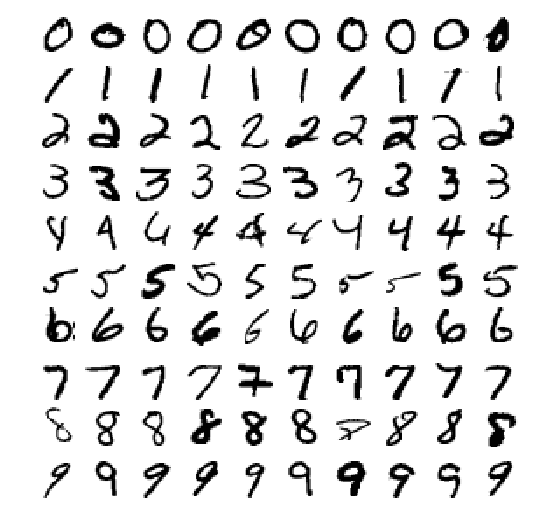

2. 创建测试集训练集

2.1 数据洗牌（注意数据的顺序敏感性）

x_train, x_test, y_train, y_test = X[:60000], X[60000:], y[:60000], y[60000:]

import numpy as np
# Randomly permute a sequence, or return a permuted range.
shuffle_index = np.random.permutation(60000)
x_train, y_train = x_train[shuffle_index], y_train[shuffle_index]

3. 训练一个二元分类器

• 例如，我们现在要识别数字5，结果要么是5要么不是5.
• SGDClassifier是一个线性分类器（默认情况下,它是一个线性SVM），它使用SGD进行训练（即，使用SGD查找损失的最小值）

from sklearn.linear_model import SGDClassifier
y_train_5 = (y_train == 5) # True for all 5s, False for all other digits.
y_test_5 = (y_test == 5)

• random_state 随机种子
  • 有一些函数每次运行的时候需要一些随机数，但是完全依靠random的话每次导入的参数都不一样，这样就无法控制变量。因此有了random_state参数，它可以生成一组随机数，但下次生成随机数的时候还是一样的随机数，而不是完全随机的。

sgd_clf = SGDClassifier(random_state=42)
sgd_clf.fit(x_train,y_train_5)
result = sgd_clf.predict([some_digit])
print(result)

D:\Anaconda3\lib\site-packages\sklearn\linear_model\stochastic_gradient.py:144: FutureWarning: max_iter and tol parameters have been added in SGDClassifier in 0.19. If both are left unset, they default to max_iter=5 and tol=None. If tol is not None, max_iter defaults to max_iter=1000. From 0.21, default max_iter will be 1000, and default tol will be 1e-3.
  FutureWarning)


[False]

4. 评估分类器

4.1 交叉验证

• StratifiedKFold类似于Kfold,比KFold的优势在于将它会按照百分比划分数据集，而不是像K折那样随意分成K份
  每个类别百分比在训练集和测试集中都是一样，这样能保证不会有某个类别的数据在训练集中而测试集中没有这种情况，
  同样不会在训练集中没有全在测试集中，这样会导致结果糟糕透顶。

from  sklearn.model_selection import  StratifiedKFold
from  sklearn.base import clone
skfolds = StratifiedKFold(n_splits=3,random_state=42)

• 对于每一“折”进行训练、预测、并输出所有“折”的平均结果

for train_index,test_index in skfolds.split(x_train,y_train_5):
    clone_clf = clone(sgd_clf)
    x_train_folds = x_train[train_index]
    y_train_folds = (y_train_5[train_index])
    x_test_fold = x_train[test_index]
    y_test_fold = (y_train_5[test_index])
    clone_clf.fit(x_train_folds,y_train_folds)
    y_pred = clone_clf.predict(x_test_fold)\
    # 将所有预测正确的结果加起来
    n_correct = sum(y_pred == y_test_fold)
    print(n_correct/len(y_pred))

0.9455


0.9636


0.95855

• 使用corss_val_score（）函数来评估SGD模型(采用k-flod交叉验证）

from sklearn.model_selection import cross_val_score
array = cross_val_score(sgd_clf,x_train,y_train_5,cv=3,scoring="accuracy")
print(array)

[0.9455  0.9636  0.95855]

• 然而，对于随意的一种分类器，理论上的正确率都会超过90%，因为6这个数字在所有数据集里面的占比就是10%
  所以，_正确率_并不是分类器性能表示的最佳指标，尤其是数据集有偏斜的时候（即某个数据量比其他多很多）

from sklearn.base import BaseEstimator
class Never5Clissifer(BaseEstimator):
    def fit (self,x,y=None):
        pass
    def predict (self,x):
        return np.zeros((len(x),1),dtype=bool)

never_5_clf = Never5Clissifer()
array = cross_val_score(never_5_clf,x_train,y_train_5,cv=3,scoring="accuracy")
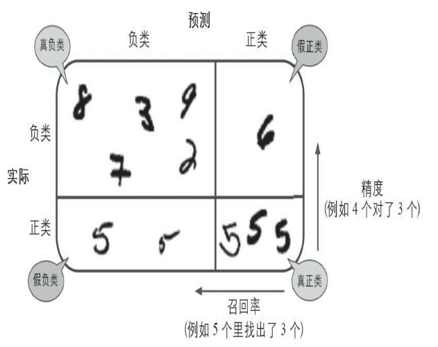
print(array)

[0.9078  0.9121  0.90905]

4.2 混淆矩阵

• 所谓混淆矩阵，就是指类别与类别之间分类错误的次数。 例如，数字3被错误分成数字5的次数会
  记录在第5行第三列。这里使用corss_val_predict来预测，返回的指是每个折叠的预测。cross_val_predict()
  通过K-fold折叠返回3组预测值，这3组测试的数据是相互隔离的，每一次预测的数据在训练期间是没见过的。

• 混淆矩阵中，行表示实际类别，列表示预测类别。如：
  \begin{matrix}
  x & y \
  z & v
  \end{matrix}
  第0行0列表示非6的图片（负类）分类成了非6的数量（成为真负类数量）；
  第0行第1列表示非6的图片分类成了6的的数量（假正类）；
  第1行第0列表示是6的图片（正类）分类成了非6的数量（假负类）；
  第1行第1列表示是6的图片分类成了6的数量（真正类）。
  所以在完美情况下，混淆矩阵只有对角线有非零值，其余均为0
  混淆矩阵图示：
  

from sklearn.model_selection import cross_val_predict
y_train_pred = cross_val_predict(sgd_clf,x_train,y_train_5,cv=3)
from sklearn.metrics import confusion_matrix
array= confusion_matrix(y_train_5,y_train_pred)
array_perfect = confusion_matrix(y_train_5,y_train_5)
print(array)
print("perfect:",array_perfect)

[[53537  1042]
 [ 1605  3816]]
perfect: [[54579     0]
          [    0  5421]]

4.3 混淆矩阵提供的信息

1.利用混淆矩阵计算分类器的精度。$$精度 = \frac{TP}{TP+FP} (TP->真正类，FP->假正类）$$

精确率是针对我们预测结果而言的，它表示的是预测为正的样本中有多少是真正的正样本。

2.利用混淆矩阵计算召回率（recall）,也叫做灵敏度（ensitivity）或者真正类率（TPR）。$$召回率=\frac{TP}{TP+FN} (FN->假负类)$$

召回率是针对我们原来的样本而言的，它表示的是样本中的正例有多少被预测正确了。

3.$F_1$分数,是精度和召回率的组合（谐波平均值，对于较低的值更高的权重，而不是传统的一视同仁）。
所以只有当召回率和精度都很高的时候，分类器的$F_1$分数才会比较高。
$$F_1 = \frac{2}{\frac{1}{精度}+{\frac{1}{召回率}}} = 2 \times \frac{精度\times召回率}{精度+召回率} = \frac{TP}{TP+\frac{FN+FP}{2}} $$

from sklearn.metrics import precision_score,recall_score
print(precision_score(y_train_5,y_train_pred))
print(recall_score(y_train_5,y_train_pred))
from sklearn.metrics import f1_score
print(f1_score(y_train_5,y_train_pred))

0.785508439687114
0.703929164360819
0.742484677497811

• 对于精确度和召回率而言，同时达到很高的水平是不太可能的。这和分类器的原理有关。分类器往往有一个阈值，高于这个阈值的就是正确的，低于的就是错误的。 当召回率越来越高时，也就是样本的正例被预测正确的概率越来越高的时候，意味着阈值越来越低，而阈值的降低势必会导致精确度的降低。所以往往要在精确度和召回率之间寻找一种平衡。下面通过sgd分类器的decision方法测试，该方法返回每个实例的分数，可用来测试阈值。

y_scores = sgd_clf.decision_function([some_digit])
print(y_scores)
threshold = 0
y_some_digit_pred = (y_scores>threshold)
print("threshold=0",y_some_digit_pred)  # 当阈值比较小的时候为True
threshold = 600000        # 提升阈值
y_some_digit_pred = (y_scores>threshold)
print("threshold=600000",y_some_digit_pred)  # 当阈值比较大的时候为False

[-19662.17519015]
threshold=0 [False]
threshold=600000 [False]

上面两个结果的变化说明，阈值的变化会改变召回率。那么如何达到准确率和召回率的平衡呢（选取最好的阈值）？

1. 首先使用cross_val_predict计算训练集中所有实例的分数。
2. 其次，使用precision_recall_curve()来计算所有可能的阈值的精度和召回率
3. 最后，使用Matplotlib绘制精度和召回率相对于阈值的函数图

y_scores = cross_val_predict(sgd_clf,x_train,y_train_5,cv=3,method="decision_function")
from sklearn.metrics import precision_recall_curve
precisions,recalls,thresholds = precision_recall_curve(y_train_5,y_scores)
def plot_precision_recall_vs_threshold(precisions,recalls,thresholds):
    plt.plot(thresholds,precisions[:-1],"r--",label="Precision") # 绘图（x,y,表示符号，标签）
    plt.plot(thresholds,recalls[:-1],"g--",label ="Recall")
    plt.xlabel("Threshold")
    plt.legend(loc="upper left") # 图例的位置
    plt.ylim([0,1])
plot_precision_recall_vs_threshold(precisions,recalls,thresholds)
plt.show()

# 指定精度/召回率的分类器
y_train_pred_90 = (y_scores>700000) # 阈值从图上找
print(precision_score(y_train_5,y_train_pred_90))
print(recall_score(y_train_5,y_train_pred_90))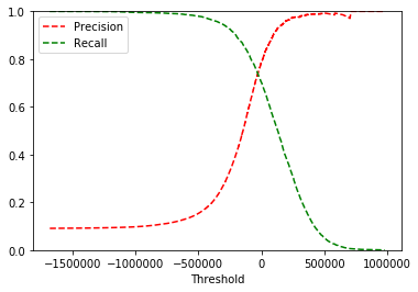

0.9714285714285714
0.006271905552481092

4.4 ROC曲线

• 一些概念：
  • 真正类率（True Positive Rate）TPR：TP/(TP/FN),表示分类器预测的正类中实际正样本占全部正样本的比例
  • 负正类率（False Positive Rate）FPR:FP/(FP+TN),表示分类器预测的正类中实际负样本占所有负样本的比例
  • 真负类率（True Negative Rate）TNR:TN/(FP+TN),表示分类器预测的负类中，实际负样本占A所有负样本的比例（TNR=1-FPR）
• ROC曲线图中，曲线上的每个点对应一个阈值
• 曲线的走势代表随着阈值的变化FPR与TPR的变化关系。
• 横轴FPR:1-TNR，FPR越大，预测结果中的正样本中负样本含量越多
• 纵轴TPR:,TPR越大，预测结果中的正样本中的正样本含量越多
• AUC(曲线下面积)，AUC的面积越大，分类器效果越好，最佳的分类器AUC等于1

from sklearn.metrics import roc_curve
fpr,tpr,thresholds = roc_curve(y_train_5,y_scores)
def plot_roc_curve(fpr,tpr,label=None):
    plt.plot(fpr,tpr,lineWidth=2,label=label)
    plt.plot([0,1],[0,1],"k--")
    plt.axis([0,1,0,1])  # 设置x轴，y轴的起始和终点
    plt.xlabel('False Positive Rate')
    plt.ylabel('True Positive Rate')
plot_roc_curve(fpr,tpr)
plt.show()
from sklearn.metrics import roc_auc_score
print(roc_auc_score(y_train_5,y_scores))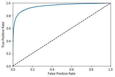

0.950155100287553

4.5 ROC曲线对比

绘制RF分类器的ROC曲线：

• RF分类器与SGD的工作方式不一样，没有decision_function()来判断阈值。但是它有dict_proda()方法。
• dict_proda返回一个数组，每一行表示一个实例，每一列表示一个类别。每个元素指的是每个实例对于每个类别的概率。

from sklearn.ensemble import RandomForestClassifier
rf_clf = RandomForestClassifier(random_state=42)
y_rf_clf = cross_val_predict(rf_clf,x_train,y_train_5,cv=3,method="predict_proba")
print(y_rf_clf)

y_scores_rf = y_rf_clf[:,1]  # 分数为正样本的概率，即取二维数组每一行的第二个数据
fpr_rf,tpr_rf,thresholds_rf = roc_curve(y_train_5,y_scores_rf)
plt.plot(fpr,tpr,"b:",label="SGD")
plot_roc_curve(fpr_rf,tpr_rf,"Random Forest")
plt.legend(loc="lower right")
plt.show()
print(roc_auc_score(y_train_5,y_scores_rf))

[[1.  0. ]
 [0.9 0.1]
 [0.9 0.1]
 ...
 [1.  0. ]
 [1.  0. ]
 [1.  0. ]]

0.9917598412633858

5.多类别分类器

多分类策略（以MNIST为例）：

• OVA: 一对多策略，训练0-9是个分类器，来一张图片经过十个分类器，取最高得分。（训练时每个分类器要训练所有数据集）
• OvO: 一对一策略，训练0-1、0-2等n（n-1）/2个分类器，每个分类器用于判断是a还是b，训练时只需要训练ab两组数据集
  所以，对于大型数据集，OvO比较好。sk-learn可以检测到我们使用二元分类进行多分类的行为，默认会使用OvA策略

sgd_clf.fit(x_train,y_train)
array = sgd_clf.predict([some_digit])
print(array)   # array([5.])
some_digit_score = sgd_clf.decision_function([some_digit])
print(some_digit_score)
# 上面代码中，sgd训练时训练了所有0-9的数据(OVA)，在内部生成了10个分类器，some_digit_score就是十个分类器的分数。在预测时，取了最高的分数给出结果
from sklearn.multiclass import OneVsOneClassifier
ovo_clf = OneVsOneClassifier(SGDClassifier(random_state=42))
ovo_clf.fit(x_train,y_train)
array = ovo_clf.predict([some_digit])
print("result:",array)                                              #结果
print("length of ovo_clf",len(ovo_clf.estimators_))                 #分类器个数
# RF的多分类策略（RD可以直接将实例分为多个类别）
rf_clf.fit(x_train,y_train)
rf_clf.predict([some_digit])
print("RF的各个类概率：",rf_clf.predict_proba([some_digit]))          #RF中各个类的概率

[5.]
[[-193260.69253369 -268272.35422435 -160594.339744   -157709.0339379
  -532207.50918753  -19662.17519015 -781920.88031095 -280417.97366431
  -856441.40614529 -552502.53905182]]


result: [5.]
length of ovo_clf 45
RF的各个类概率： [[0.1 0.  0.  0.1 0.  0.8 0.  0.  0.  0. ]]

5.1 多分类性能测试

array = cross_val_score(sgd_clf,x_train,y_train,cv=3,scoring="accuracy")
print("3折交叉检验：",array)
from sklearn.preprocessing import StandardScaler
scaler = StandardScaler()
x_train_scaler = scaler.fit_transform(x_train.astype(np.float64))  # astype:数据类型转换
array = cross_val_score(sgd_clf,x_train_scaler,y_train,cv=3,scoring="accuracy")
print("特征缩放后的准确率：",array)

3折交叉检验： [0.85472905 0.86074304 0.86738011]


特征缩放后的准确率： [0.90826835 0.90894545 0.91053658]

5.2 错误分析

# 生成混淆矩阵
y_train_pred = cross_val_predict(sgd_clf,x_train_scaler,y_train,cv=3)
conf_mx = confusion_matrix(y_train,y_train_pred)
print(conf_mx)
plt.matshow(conf_mx,cmap=plt.cm.gray)
plt.show()

[[5733    2   22    8    9   50   47    7   42    3]
 [   2 6490   44   25    6   41    8   13  100   13]
 [  59   37 5319   97   83   26   99   62  159   17]
 [  43   42  128 5345    1  232   32   53  142  113]
 [  20   25   39    8 5385    9   49   32   73  202]
 [  70   38   32  212   80 4574  112   27  173  103]
 [  36   25   44    2   39  104 5624    4   40    0]
 [  25   21   62   24   64   12    4 5793   12  248]
 [  52  156   67  145   17  158   50   26 5023  157]
 [  44   33   24   80  172   38    2  210   77 5269]]

# 计算每个类别的错误率
row_sums = conf_mx.sum(axis=1, keepdims=True)  # keepdims用来保持矩阵的多维特征，也就是sum操作后还是跟混淆矩阵一样的二维矩阵）
norm_conf_mx = conf_mx / row_sums

# 用0填充对角线，只保留错误。
np.fill_diagonal(norm_conf_mx,0)               # 填充任意维度矩阵的主对角线
plt.matshow(norm_conf_mx,cmap=plt.cm.gray)
plt.show()
# 结果分析：每一行代表实际类别，每一列代表被分类的类别。越暗说明越正确。比如第4行的第9列很亮，表示
# 有很多的4被错误分成了9. 同样，有不少8被错误分为了1、3、5、9等数字。混淆矩阵可以直观的看出来每个
# 分类的具体情况。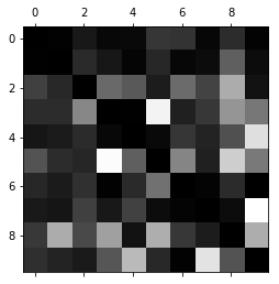

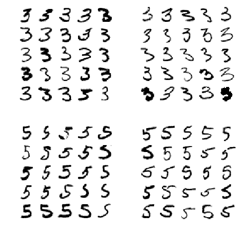
# 组合显示样例图片
cl_a, cl_b = 3, 5
x_aa = x_train[(y_train == cl_a) & (y_train_pred == cl_a)]
x_ab = x_train[(y_train == cl_a) & (y_train_pred == cl_b)]
x_ba = x_train[(y_train == cl_b) & (y_train_pred == cl_a)]
x_bb = x_train[(y_train == cl_b) & (y_train_pred == cl_b)]

plt.figure(figsize=(8, 8))
plt.subplot(221)                                # subplot：组合很多小图，放到大图里面显示
plot_digits(x_aa[:25], images_per_row=5)
plt.subplot(222)
plot_digits(x_ab[:25], images_per_row=5)
plt.subplot(223)
plot_digits(x_ba[:25], images_per_row=5)
plt.subplot(224)
plot_digits(x_bb[:25], images_per_row=5)
plt.show()

6.多标签分类

from sklearn.neighbors import KNeighborsClassifier
y_train_large = (y_train>=7)                      # 标签1：数字是否大于等于7
y_train_odd = (y_train%2==1)                      # 标签2：数字是否为奇数
y_multilabel = np.c_[y_train_large,y_train_odd]

knn_clf = KNeighborsClassifier()                  # 训练一个KNN分类器
knn_clf.fit(x_train,y_multilabel)
array = knn_clf.predict([some_digit])
print(array)

[[False  True]]

6.1 多标签分类评价： 平均$F_1$分数

y_train_knn_pred = cross_val_predict(knn_clf,x_train,y_train,cv=3)
f1_score(y_train,y_train_knn_pred,average="macro")

7.多输出分类

noise = np.random.randint(0, 100, (len(x_train), 784))      # 给图片加噪声
X_train_mod = x_train + noise
noise = np.random.randint(0, 100, (len(x_test), 784))
X_test_mod = x_test + noise
y_train_mod = x_train
y_test_mod = x_test
some_index = 5500
plt.subplot(121); plot_digits(X_test_mod[some_index])
plt.subplot(122); plot_digits(y_test_mod[some_index])
plt.show()

knn_clf.fit(X_train_mod, y_train_mod)
clean_digit = knn_clf.predict([X_test_mod[some_index]])
plot_digits(clean_digit)