1.import 模块
import os
import tarfile
from six.moves import urllib
import pandas as pd
pd.set_option('display.width', None)
import matplotlib.pyplot as plt
import numpy as np
import hashlib
2.获取数据模块
DOWNLOAD_ROOT = "https://raw.githubusercontent.com/ageron/handson-ml/master/"
HOUSING_PATH = "datasets/housing"
HOUSING_URL = DOWNLOAD_ROOT + HOUSING_PATH + "/housing.tgz"
print(HOUSING_URL)
https://raw.githubusercontent.com/ageron/handson-ml/master/datasets/housing/housing.tgzdef fetch_housing_data(housing_url=HOUSING_URL, housing_path=HOUSING_PATH):
if not os.path.isdir(housing_path):
os.makedirs(housing_path)
tgz_path = os.path.join(housing_path, "housing.tgz")
urllib.request.urlretrieve(housing_url, tgz_path)
housing_tgz = tarfile.open(tgz_path)
housing_tgz.extractall(path=housing_path)
housing_tgz.close()
def load_housing_data(housing_path=HOUSING_PATH): # 加载数据函数
csv_path = os.path.join(housing_path, "housing.csv")
print(csv_path)
return pd.read_csv(csv_path) # 返回一个pandas DataFrame对象
2.1查看数据
housing = load_housing_data()
print("---" * 20)
print("         查看pandas DataFrame对象的头部(前5行")
print("---" * 20)
print(housing.head())  # 查看pandas DataFrame对象的头部
print("---" * 20)
print("         查看pandas DataFrame的具体信息")
print("---" * 20)
print(housing.info())  # 查看pandas DataFrmae的具体信息
print("---" * 20)
print("         查看pandas DataFrame中ocean_proximity字段的分类信息")
print("---" * 20)
print(housing["ocean_proximity"].value_counts())
print("---" * 20)
print("         查看具体数值属性的摘要")
print("---" * 20)
print(housing.describe())
datasets/housing\housing.csv
------------------------------------------------------------
         查看pandas DataFrame对象的头部(前5行
------------------------------------------------------------
   longitude  latitude  housing_median_age  total_rooms  total_bedrooms  \
0    -122.23     37.88                41.0        880.0           129.0
1    -122.22     37.86                21.0       7099.0          1106.0
2    -122.24     37.85                52.0       1467.0           190.0
3    -122.25     37.85                52.0       1274.0           235.0
4    -122.25     37.85                52.0       1627.0           280.0

   population  households  median_income  median_house_value ocean_proximity
0       322.0       126.0         8.3252            452600.0        NEAR BAY
1      2401.0      1138.0         8.3014            358500.0        NEAR BAY
2       496.0       177.0         7.2574            352100.0        NEAR BAY
3       558.0       219.0         5.6431            341300.0        NEAR BAY
4       565.0       259.0         3.8462            342200.0        NEAR BAY
------------------------------------------------------------
         查看pandas DataFrame的具体信息
------------------------------------------------------------
<class 'pandas.core.frame.DataFrame'>
RangeIndex: 20640 entries, 0 to 20639
Data columns (total 10 columns):
longitude             20640 non-null float64
latitude              20640 non-null float64
housing_median_age    20640 non-null float64
total_rooms           20640 non-null float64
total_bedrooms        20433 non-null float64
population            20640 non-null float64
households            20640 non-null float64
median_income         20640 non-null float64
median_house_value    20640 non-null float64
ocean_proximity       20640 non-null object
dtypes: float64(9), object(1)
memory usage: 1.6+ MB
None
------------------------------------------------------------
         查看pandas DataFrame中ocean_proximity字段的分类信息
------------------------------------------------------------
<1H OCEAN     9136
INLAND        6551
NEAR OCEAN    2658
NEAR BAY      2290
ISLAND           5
Name: ocean_proximity, dtype: int64
------------------------------------------------------------
         查看具体数值属性的摘要
------------------------------------------------------------
          longitude      latitude  housing_median_age   total_rooms  \
count  20640.000000  20640.000000        20640.000000  20640.000000
mean    -119.569704     35.631861           28.639486   2635.763081
std        2.003532      2.135952           12.585558   2181.615252
min     -124.350000     32.540000            1.000000      2.000000
25%     -121.800000     33.930000           18.000000   1447.750000
50%     -118.490000     34.260000           29.000000   2127.000000
75%     -118.010000     37.710000           37.000000   3148.000000
max     -114.310000     41.950000           52.000000  39320.000000

       total_bedrooms    population    households  median_income  \
count    20433.000000  20640.000000  20640.000000   20640.000000
mean       537.870553   1425.476744    499.539680       3.870671
std        421.385070   1132.462122    382.329753       1.899822
min          1.000000      3.000000      1.000000       0.499900
25%        296.000000    787.000000    280.000000       2.563400
50%        435.000000   1166.000000    409.000000       3.534800
75%        647.000000   1725.000000    605.000000       4.743250
max       6445.000000  35682.000000   6082.000000      15.000100

       median_house_value
count        20640.000000
mean        206855.816909
std         115395.615874
min          14999.000000
25%         119600.000000
50%         179700.000000
75%         264725.000000
max         500001.000000
bins : integer or array_like, optional
这个参数指定bin(箱子)的个数,也就是总共有几条条状图
igsize The size in inches of the figure to create. Uses the value in matplotlib.rcParams by default.这个参数指创建图形的大小
housing.hist(bins=50, figsize=(20, 20)) # 绘制housing数据的直方图
array([[<matplotlib.axes._subplots.AxesSubplot object at 0x000002393010CEF0>,
        <matplotlib.axes._subplots.AxesSubplot object at 0x000002393040C780>,
        <matplotlib.axes._subplots.AxesSubplot object at 0x0000023930667A90>],
       [<matplotlib.axes._subplots.AxesSubplot object at 0x0000023930691DA0>,
        <matplotlib.axes._subplots.AxesSubplot object at 0x00000239306C40F0>,
        <matplotlib.axes._subplots.AxesSubplot object at 0x00000239306C4128>],
       [<matplotlib.axes._subplots.AxesSubplot object at 0x00000239307156D8>,
        <matplotlib.axes._subplots.AxesSubplot object at 0x000002393073E9E8>,
        <matplotlib.axes._subplots.AxesSubplot object at 0x0000023930769CF8>]],
      dtype=object)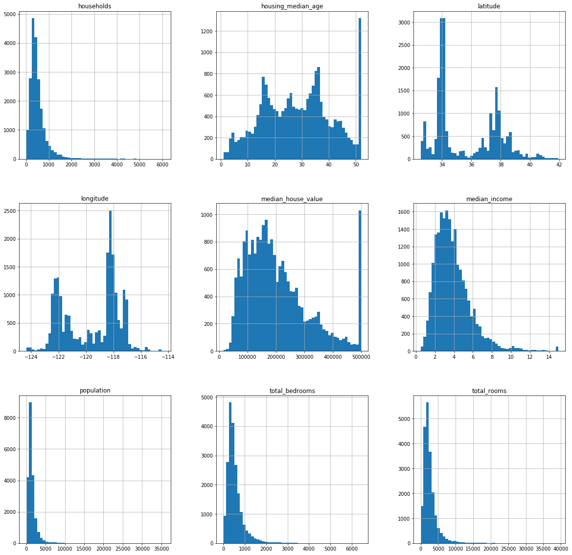
3. 使用随机抽样创建测试集
def split_train_test(data, test_ratio):
    shuffled_indices = np.random.permutation(len(data))  # 随机洗牌
    test_set_size = int(len(data) * test_ratio)
    test_indices = shuffled_indices[:test_set_size]  # 取test_set
    train_indices = shuffled_indices[test_set_size:]  # 取train_set
    return data.iloc[train_indices], data.iloc[test_indices]


train_set, test_set = split_train_test(housing, 0.2)
print(len(train_set), "train +", len(test_set), "test")
16512 train + 4128 testtrain_set和test_set分割后的问题:
- 按如上办法分割出20%的test_set,但是这个方法有一个问题,就是每一次运行程序时的test_set和train_set的数据集都不一样,这样数据分析的时候就会有问题。
解决方案:
- Option1:在程序第一次运行时保存test_set和train_set,以后每次运行都加载它们。
- Option2:在每次调用random.permutation生成随机序列的时候都生成一个随机索引,比如:np.random.seed(),每次执行方法查找索引找数据集。
这两个方法同样有问题,就是每当数据更新时,程序要重新开始运行,所有的从头开始。所以有Option3。- Option3:对每一个实例都用一个标识符来决定是否让他加入数据集中。如:给每一个实例都加一个唯一的标识符,计算每个标识符的hash值,取hash的最后一个字节,该值小于51(256的20%)就让他加入测试集。注:使用这个方法要保证在加入新数据时各个数据的index不变,否则就没有意义了。
3.1 Option3 实现
def test_set_check(identifer, test_ratio, hash):
    return hash(np.int64(identifer)).digest()[-1] < 256 * test_ratio  # 检查最后一位


def split_train_test_by_id(data, test_radio, id_colum, hash=hashlib.md5):
    ids = data[id_colum]
    int_test_set = ids.apply(lambda id_: test_set_check(id_, test_radio, hash))
    return data.loc[~int_test_set], data.loc[
        int_test_set]  # loc:通过行标签索引数据 iloc:通过行号索引行数据 ix:通过行标签或行号索引数据(基于loc和iloc的混合)


housing_with_id = housing.reset_index()  # 给数据加colum->index
'''
train_set,test_set=split_train_test_by_id(housing_with_id,0.2,"index")  # 使用普通序列作为标识符
'''
housing_with_id["id"] = housing["longitude"] * 1000 +     housing["latitude"]  # 使用经纬度作为标识符(可以保证标识符不变)
train_set_by_id, test_set = split_train_test_by_id(housing_with_id, 0.2, "id")
- 在这个数据集中有部分房屋数据的经纬度是一样的,所以一部分的ID也是一样的位置信息实际上是相当粗粒度的,许多区域可能会拥有完全相同的ID,结果就是它们会被纳入同一个集合(测试集或者训练集)。而这有可能会导致一些抽样偏差。
print("---" * 20)
print("         加入标识符的数据:")
print("---" * 20)
print(housing_with_id)
------------------------------------------------------------
加入标识符的数据:
------------------------------------------------------------
index longitude latitude housing_median_age total_rooms \
0 0 -122.23 37.88 41.0 880.0
1 1 -122.22 37.86 21.0 7099.0
2 2 -122.24 37.85 52.0 1467.0
3 3 -122.25 37.85 52.0 1274.0
4 4 -122.25 37.85 52.0 1627.0
5 5 -122.25 37.85 52.0 919.0
6 6 -122.25 37.84 52.0 2535.0
7 7 -122.25 37.84 52.0 3104.0
8 8 -122.26 37.84 42.0 2555.0
9 9 -122.25 37.84 52.0 3549.0
10 10 -122.26 37.85 52.0 2202.0
11 11 -122.26 37.85 52.0 3503.0
12 12 -122.26 37.85 52.0 2491.0
13 13 -122.26 37.84 52.0 696.0
14 14 -122.26 37.85 52.0 2643.0
15 15 -122.26 37.85 50.0 1120.0
16 16 -122.27 37.85 52.0 1966.0
17 17 -122.27 37.85 52.0 1228.0
18 18 -122.26 37.84 50.0 2239.0
19 19 -122.27 37.84 52.0 1503.0
20 20 -122.27 37.85 40.0 751.0
21 21 -122.27 37.85 42.0 1639.0
22 22 -122.27 37.84 52.0 2436.0
23 23 -122.27 37.84 52.0 1688.0
24 24 -122.27 37.84 52.0 2224.0
25 25 -122.28 37.85 41.0 535.0
26 26 -122.28 37.85 49.0 1130.0
27 27 -122.28 37.85 52.0 1898.0
28 28 -122.28 37.84 50.0 2082.0
29 29 -122.28 37.84 52.0 729.0
... ... ... ... ... ...
20610 20610 -121.56 39.10 28.0 2130.0
20611 20611 -121.55 39.10 27.0 1783.0
20612 20612 -121.56 39.08 26.0 1377.0
20613 20613 -121.55 39.09 31.0 1728.0
20614 20614 -121.54 39.08 26.0 2276.0
20615 20615 -121.54 39.08 23.0 1076.0
20616 20616 -121.53 39.08 15.0 1810.0
20617 20617 -121.53 39.06 20.0 561.0
20618 20618 -121.55 39.06 25.0 1332.0
20619 20619 -121.56 39.01 22.0 1891.0
20620 20620 -121.48 39.05 40.0 198.0
20621 20621 -121.47 39.01 37.0 1244.0
20622 20622 -121.44 39.00 20.0 755.0
20623 20623 -121.37 39.03 32.0 1158.0
20624 20624 -121.41 39.04 16.0 1698.0
20625 20625 -121.52 39.12 37.0 102.0
20626 20626 -121.43 39.18 36.0 1124.0
20627 20627 -121.32 39.13 5.0 358.0
20628 20628 -121.48 39.10 19.0 2043.0
20629 20629 -121.39 39.12 28.0 10035.0
20630 20630 -121.32 39.29 11.0 2640.0
20631 20631 -121.40 39.33 15.0 2655.0
20632 20632 -121.45 39.26 15.0 2319.0
20633 20633 -121.53 39.19 27.0 2080.0
20634 20634 -121.56 39.27 28.0 2332.0
20635 20635 -121.09 39.48 25.0 1665.0
20636 20636 -121.21 39.49 18.0 697.0
20637 20637 -121.22 39.43 17.0 2254.0
20638 20638 -121.32 39.43 18.0 1860.0
20639 20639 -121.24 39.37 16.0 2785.0
total_bedrooms population households median_income \
0 129.0 322.0 126.0 8.3252
1 1106.0 2401.0 1138.0 8.3014
2 190.0 496.0 177.0 7.2574
3 235.0 558.0 219.0 5.6431
4 280.0 565.0 259.0 3.8462
5 213.0 413.0 193.0 4.0368
6 489.0 1094.0 514.0 3.6591
7 687.0 1157.0 647.0 3.1200
8 665.0 1206.0 595.0 2.0804
9 707.0 1551.0 714.0 3.6912
10 434.0 910.0 402.0 3.2031
11 752.0 1504.0 734.0 3.2705
12 474.0 1098.0 468.0 3.0750
13 191.0 345.0 174.0 2.6736
14 626.0 1212.0 620.0 1.9167
15 283.0 697.0 264.0 2.1250
16 347.0 793.0 331.0 2.7750
17 293.0 648.0 303.0 2.1202
18 455.0 990.0 419.0 1.9911
19 298.0 690.0 275.0 2.6033
20 184.0 409.0 166.0 1.3578
21 367.0 929.0 366.0 1.7135
22 541.0 1015.0 478.0 1.7250
23 337.0 853.0 325.0 2.1806
24 437.0 1006.0 422.0 2.6000
25 123.0 317.0 119.0 2.4038
26 244.0 607.0 239.0 2.4597
27 421.0 1102.0 397.0 1.8080
28 492.0 1131.0 473.0 1.6424
29 160.0 395.0 155.0 1.6875
... ... ... ... ...
20610 484.0 1195.0 439.0 1.3631
20611 441.0 1163.0 409.0 1.2857
20612 289.0 761.0 267.0 1.4934
20613 365.0 1167.0 384.0 1.4958
20614 460.0 1455.0 474.0 2.4695
20615 216.0 724.0 197.0 2.3598
20616 441.0 1157.0 375.0 2.0469
20617 109.0 308.0 114.0 3.3021
20618 247.0 726.0 226.0 2.2500
20619 340.0 1023.0 296.0 2.7303
20620 41.0 151.0 48.0 4.5625
20621 247.0 484.0 157.0 2.3661
20622 147.0 457.0 157.0 2.4167
20623 244.0 598.0 227.0 2.8235
20624 300.0 731.0 291.0 3.0739
20625 17.0 29.0 14.0 4.1250
20626 184.0 504.0 171.0 2.1667
20627 65.0 169.0 59.0 3.0000
20628 421.0 1018.0 390.0 2.5952
20629 1856.0 6912.0 1818.0 2.0943
20630 505.0 1257.0 445.0 3.5673
20631 493.0 1200.0 432.0 3.5179
20632 416.0 1047.0 385.0 3.1250
20633 412.0 1082.0 382.0 2.5495
20634 395.0 1041.0 344.0 3.7125
20635 374.0 845.0 330.0 1.5603
20636 150.0 356.0 114.0 2.5568
20637 485.0 1007.0 433.0 1.7000
20638 409.0 741.0 349.0 1.8672
20639 616.0 1387.0 530.0 2.3886
median_house_value ocean_proximity id
0 452600.0 NEAR BAY -122192.12
1 358500.0 NEAR BAY -122182.14
2 352100.0 NEAR BAY -122202.15
3 341300.0 NEAR BAY -122212.15
4 342200.0 NEAR BAY -122212.15
5 269700.0 NEAR BAY -122212.15
6 299200.0 NEAR BAY -122212.16
7 241400.0 NEAR BAY -122212.16
8 226700.0 NEAR BAY -122222.16
9 261100.0 NEAR BAY -122212.16
10 281500.0 NEAR BAY -122222.15
11 241800.0 NEAR BAY -122222.15
12 213500.0 NEAR BAY -122222.15
13 191300.0 NEAR BAY -122222.16
14 159200.0 NEAR BAY -122222.15
15 140000.0 NEAR BAY -122222.15
16 152500.0 NEAR BAY -122232.15
17 155500.0 NEAR BAY -122232.15
18 158700.0 NEAR BAY -122222.16
19 162900.0 NEAR BAY -122232.16
20 147500.0 NEAR BAY -122232.15
21 159800.0 NEAR BAY -122232.15
22 113900.0 NEAR BAY -122232.16
23 99700.0 NEAR BAY -122232.16
24 132600.0 NEAR BAY -122232.16
25 107500.0 NEAR BAY -122242.15
26 93800.0 NEAR BAY -122242.15
27 105500.0 NEAR BAY -122242.15
28 108900.0 NEAR BAY -122242.16
29 132000.0 NEAR BAY -122242.16
... ... ... ...
20610 45500.0 INLAND -121520.90
20611 47000.0 INLAND -121510.90
20612 48300.0 INLAND -121520.92
20613 53400.0 INLAND -121510.91
20614 58000.0 INLAND -121500.92
20615 57500.0 INLAND -121500.92
20616 55100.0 INLAND -121490.92
20617 70800.0 INLAND -121490.94
20618 63400.0 INLAND -121510.94
20619 99100.0 INLAND -121520.99
20620 100000.0 INLAND -121440.95
20621 77500.0 INLAND -121430.99
20622 67000.0 INLAND -121401.00
20623 65500.0 INLAND -121330.97
20624 87200.0 INLAND -121370.96
20625 72000.0 INLAND -121480.88
20626 93800.0 INLAND -121390.82
20627 162500.0 INLAND -121280.87
20628 92400.0 INLAND -121440.90
20629 108300.0 INLAND -121350.88
20630 112000.0 INLAND -121280.71
20631 107200.0 INLAND -121360.67
20632 115600.0 INLAND -121410.74
20633 98300.0 INLAND -121490.81
20634 116800.0 INLAND -121520.73
20635 78100.0 INLAND -121050.52
20636 77100.0 INLAND -121170.51
20637 92300.0 INLAND -121180.57
20638 84700.0 INLAND -121280.57
20639 89400.0 INLAND -121200.63
[20640 rows x 12 columns]3.2 使用sk-learn生成随机数据集
一个函数包含从split_train_test到这一行以上的所有内容。。。。
from sklearn.model_selection import train_test_split

train_set, test_set = train_test_split(housing, test_size=0.2, random_state=42)
# random就是Option2 生成随机索引
print(test_set)
       longitude  latitude  housing_median_age  total_rooms  total_bedrooms  \
20046    -119.01     36.06                25.0       1505.0             NaN
3024     -119.46     35.14                30.0       2943.0             NaN
15663    -122.44     37.80                52.0       3830.0             NaN
20484    -118.72     34.28                17.0       3051.0             NaN
9814     -121.93     36.62                34.0       2351.0             NaN
13311    -117.61     34.08                12.0       4427.0             NaN
7113     -118.02     33.89                36.0       1375.0             NaN
7668     -118.08     33.92                38.0       1335.0             NaN
18246    -122.08     37.39                 4.0       2292.0             NaN
5723     -118.23     34.18                45.0       2332.0             NaN
20069    -120.37     38.01                30.0        473.0             NaN
6835     -118.12     34.08                35.0       2248.0             NaN
11351    -117.91     33.76                20.0       4413.0             NaN
20267    -119.19     34.20                18.0       3620.0             NaN
7097     -117.98     33.92                27.0       3700.0             NaN
6298     -117.91     34.02                22.0       6269.0             NaN
696      -122.10     37.69                41.0        746.0             NaN
19607    -121.02     37.48                26.0        467.0             NaN
14173    -117.05     32.75                36.0       2024.0             NaN
19638    -120.97     37.43                27.0       1380.0             NaN
18332    -122.16     37.45                47.0       4234.0             NaN
4691     -118.37     34.07                50.0       2519.0             NaN
2323     -119.73     36.83                 8.0       3602.0             NaN
16880    -122.39     37.59                32.0       4497.0             NaN
14521    -117.14     32.90                16.0       3217.0             NaN
19833    -119.38     36.53                38.0       1281.0             NaN
8383     -118.36     33.96                26.0       3543.0             NaN
2647     -124.13     40.55                38.0        544.0             NaN
1456     -121.98     37.96                22.0       2987.0             NaN
5678     -118.30     33.72                35.0       2790.0             NaN
...          ...       ...                 ...          ...             ...
146      -122.22     37.81                52.0       1971.0           335.0
4989     -118.31     34.00                47.0       1551.0           362.0
16215    -121.34     37.96                27.0       1839.0           442.0
241      -122.21     37.78                52.0       1477.0           300.0
18746    -122.34     40.51                16.0       2247.0           502.0
3595     -118.49     34.24                35.0       2707.0           446.0
8404     -118.36     33.93                30.0       1132.0           347.0
10360    -117.67     33.57                18.0       1614.0           210.0
5714     -118.23     34.21                50.0        309.0            47.0
12401    -116.31     33.65                 8.0       3079.0           558.0
1952     -120.81     38.73                38.0       2005.0           385.0
15800    -122.44     37.76                52.0       2959.0           683.0
1594     -122.12     37.91                34.0       5683.0           755.0
9161     -118.49     34.42                23.0       4166.0           756.0
8478     -118.31     33.93                35.0       1580.0           266.0
10087    -117.97     33.94                36.0       1870.0           338.0
2680     -115.51     32.99                20.0       1402.0           287.0
844      -122.07     37.58                16.0       1644.0           251.0
4779     -118.32     34.04                47.0       1989.0           532.0
11919    -117.42     33.95                32.0       4251.0           848.0
4653     -118.33     34.06                52.0       1368.0           231.0
1783     -122.36     37.94                26.0       1540.0           343.0
7608     -118.26     33.88                40.0        519.0           102.0
0        -122.23     37.88                41.0        880.0           129.0
10155    -117.89     33.89                17.0       1671.0           192.0
15362    -117.22     33.36                16.0       3165.0           482.0
16623    -120.83     35.36                28.0       4323.0           886.0
18086    -122.05     37.31                25.0       4111.0           538.0
2144     -119.76     36.77                36.0       2507.0           466.0
3665     -118.37     34.22                17.0       1787.0           463.0

       population  households  median_income  median_house_value  \
20046      1392.0       359.0         1.6812             47700.0
3024       1565.0       584.0         2.5313             45800.0
15663      1310.0       963.0         3.4801            500001.0
20484      1705.0       495.0         5.7376            218600.0
9814       1063.0       428.0         3.7250            278000.0
13311      2400.0       843.0         4.7147            158700.0
7113        670.0       221.0         5.0839            198200.0
7668       1011.0       269.0         3.6908            157500.0
18246      1050.0       584.0         4.8036            340000.0
5723        943.0       339.0         8.1132            446600.0
20069       242.0        93.0         2.5417            123200.0
6835       1762.0       622.0         3.0000            253900.0
11351      4818.0      1063.0         2.8594            215100.0
20267      3171.0       779.0         3.3409            220500.0
7097       1793.0       552.0         5.3668            219800.0
6298       5587.0      1251.0         3.8201            136200.0
696         387.0       161.0         3.9063            178400.0
19607       244.0        83.0         4.1346            187500.0
14173      1030.0       390.0         3.8233            139800.0
19638       810.0       262.0         2.1875            137500.0
18332      1808.0      1093.0         4.2297            425000.0
4691       1117.0       516.0         4.3667            405600.0
2323       1959.0       580.0         5.3478            138800.0
16880      1846.0       715.0         6.1323            500001.0
14521      2054.0       687.0         4.2234            162100.0
19833      1423.0       293.0         1.9602             51400.0
8383       2742.0       951.0         2.5504            151300.0
2647        240.0        91.0         3.2500             94800.0
1456       1420.0       540.0         3.6500            204100.0
5678       1167.0       441.0         6.2028            361500.0
...           ...         ...            ...                 ...
146         765.0       308.0         6.5217            273700.0
4989       1329.0       322.0         1.9792            116400.0
16215      2010.0       416.0         2.1284             59400.0
241        1065.0       269.0         1.8472            137000.0
18746      1206.0       463.0         1.9946            119200.0
3595       1224.0       445.0         5.2939            244200.0
8404       1433.0       341.0         2.6800            170000.0
10360       692.0       209.0         7.9294            280300.0
5714        121.0        45.0         6.2130            285000.0
12401      1572.0       474.0         4.5938            102600.0
1952        882.0       353.0         2.5104            120500.0
15800      1145.0       666.0         4.2222            361600.0
1594       1962.0       723.0         8.3678            455300.0
9161       2082.0       743.0         4.4107            213400.0
8478        926.0       282.0         5.0653            158000.0
10087       947.0       324.0         4.1205            217000.0
2680       1104.0       317.0         1.9088             63700.0
844        1033.0       267.0         6.5116            244300.0
4779       1430.0       519.0         1.8333            151100.0
11919      2494.0       798.0         2.8173            110800.0
4653        737.0       248.0         8.3617            433800.0
1783       1007.0       338.0         1.3365             72900.0
7608        330.0        95.0         3.0972            108500.0
0           322.0       126.0         8.3252            452600.0
10155       678.0       206.0        13.1107            467600.0
15362      1351.0       452.0         4.6050            263300.0
16623      1650.0       705.0         2.7266            266800.0
18086      1585.0       568.0         9.2298            500001.0
2144       1227.0       474.0         2.7850             72300.0
3665       1671.0       448.0         3.5521            151500.0

      ocean_proximity
20046          INLAND
3024           INLAND
15663        NEAR BAY
20484       <1H OCEAN
9814       NEAR OCEAN
13311          INLAND
7113        <1H OCEAN
7668        <1H OCEAN
18246        NEAR BAY
5723        <1H OCEAN
20069          INLAND
6835        <1H OCEAN
11351       <1H OCEAN
20267      NEAR OCEAN
7097        <1H OCEAN
6298        <1H OCEAN
696          NEAR BAY
19607          INLAND
14173      NEAR OCEAN
19638          INLAND
18332        NEAR BAY
4691        <1H OCEAN
2323           INLAND
16880      NEAR OCEAN
14521       <1H OCEAN
19833          INLAND
8383        <1H OCEAN
2647        <1H OCEAN
1456           INLAND
5678       NEAR OCEAN
...               ...
146          NEAR BAY
4989        <1H OCEAN
16215          INLAND
241          NEAR BAY
18746          INLAND
3595        <1H OCEAN
8404        <1H OCEAN
10360       <1H OCEAN
5714        <1H OCEAN
12401          INLAND
1952           INLAND
15800        NEAR BAY
1594         NEAR BAY
9161        <1H OCEAN
8478        <1H OCEAN
10087       <1H OCEAN
2680           INLAND
844          NEAR BAY
4779        <1H OCEAN
11919          INLAND
4653        <1H OCEAN
1783         NEAR BAY
7608        <1H OCEAN
0            NEAR BAY
10155       <1H OCEAN
15362       <1H OCEAN
16623      NEAR OCEAN
18086       <1H OCEAN
2144           INLAND
3665        <1H OCEAN

[4128 rows x 10 columns]- 在数据量很大的情况下使用随机抽样通常都能有效建立test_set和train_set 但是,在数据量不大的情况下随机抽样就会有问题。比如要调查某件事跟性别有关,当地男女比例就是一个很重要的信息,然而,如果我们只有100的志愿者可以调查,随机抽样20%的时候,抽到1个女的,19个男的,这个test的结果就会有很大的倾斜。 所以,在数据量小的情况下使用分层抽样保证相应的比例,训练效果会更好。
4.数据分析
房价关联收入 --> 对收入分层抽样,按收入类别预测房价
# Return the ceiling of the input, element-wise.
housing["income_cat"] = np.ceil(housing["median_income"] / 1.5)
housing["income_cat"].where(housing["income_cat"] < 5, 5.0, inplace=True)
from sklearn.model_selection import StratifiedShuffleSplit
split = StratifiedShuffleSplit(
    n_splits=1, test_size=0.2, random_state=42)  # 分层采样
# 尝试更多的各个属性的组合 发现更多的数据关联
housing["room_per_household"] = housing["total_rooms"] / housing["households"]
housing["bedrooms_per_house"] = housing["total_bedrooms"] / housing["total_rooms"]
housing["population_per_household"] = housing["population"] / housing["households"]
corr_matrix = housing.corr()
print(corr_matrix["median_house_value"].sort_values(ascending=False))median_house_value 1.000000
median_income 0.688075
income_cat 0.643892
room_per_household 0.151948
total_rooms 0.134153
housing_median_age 0.105623
households 0.065843
total_bedrooms 0.049686
population_per_household -0.023737
population -0.024650
longitude -0.045967
latitude -0.144160
bedrooms_per_house -0.255880
Name: median_house_value, dtype: float64分层采样实例:
- 假设
housing["income_cat"]=[1,1,1,1,1,2,2,22,2,2,2,2,2,2]也就是4个1,10个2,1所占的比例为1/3,2占的比例为2/3;则经过split.split(housing, housing["income_cat"])后strat_train_set [“income_cat”]和strat_test_set[“income_cat”]中1和2,所占的比例相同,分别为1/2,和2/3.也就是说,strat_train_set [“income_cat”]中有4个1,8个2;而strat_test_set[“income_cat”]中有1个1,2个2
for train_index, test_index in split.split(housing, housing["income_cat"]):
    strat_train_set = housing.loc[train_index]
    strat_test_set = housing.loc[test_index]
print(housing["income_cat"].value_counts() / len(housing))
3.0    0.350581
2.0    0.318847
4.0    0.176308
5.0    0.114438
1.0    0.039826
Name: income_cat, dtype: float64
丢弃income_cat属性
- 沿着行的方向扫描数据(axis=1),丢弃所有行里面income_cat下的数据(也就删除了一列)
for set in (strat_test_set, strat_train_set):
    set.drop(["income_cat"], axis=1, inplace=True)
4.1数据可视化分析
housing = strat_train_set.copy()  # 创建一个用于探索的探索集
# housing.plot(kind = "scatter",x="longitude",y="latitude"); # 绘制经纬度的散点图
housing.plot(kind="scatter", x="longitude",
             y="latitude", alpha=0.1)  # 突出散点图的高密度区域
<matplotlib.axes._subplots.AxesSubplot at 0x23933a6f208>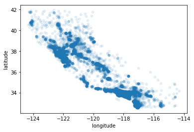
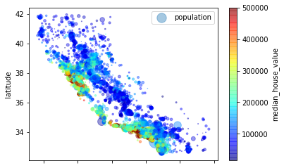
用人口和收入标识的散点图:
- 每个⚪的大小代表了人口的数量(参数s),颜色代表价格(参数c)
- s表示点点的大小,c就是color jet是一种颜色体系
housing.plot(kind="scatter", x="longitude", y="latitude", alpha=0.4,
             s=housing["population"] / 100, label="population",
             c="median_house_value", cmap=plt.get_cmap("jet"), colorbar=True)
<matplotlib.axes._subplots.AxesSubplot at 0x239301d4da0>
使用corr计算所有参数的标准相关系数(皮尔逊相关系数):
- 相关系数仅测量线性相关性(“如果x上升,则y上升/下降”),非线性的相关性无法被检测出
- 相关系数矩阵中,要重点注意的是正相关与负相关数值大的,靠近的0的可以不考虑
corr_matrix = housing.corr()
print(corr_matrix["median_house_value"].sort_values(ascending=False))
median_house_value          1.000000
median_income               0.687160
room_per_household          0.146285
total_rooms                 0.135097
housing_median_age          0.114110
households                  0.064506
total_bedrooms              0.047689
population_per_household   -0.021985
population                 -0.026920
longitude                  -0.047432
latitude                   -0.142724
bedrooms_per_house         -0.259984
Name: median_house_value, dtype: float64
4.11 使用pandas的scatter_matrix绘制相关性
from pandas.plotting import scatter_matrix
attributes = ["median_house_value", "median_income",
              "total_rooms", "housing_median_age"]
# 根据4个属性,绘制一个4X4的相关性散点图。大小大小为12,8
scatter_matrix(housing[attributes], figsize=(12, 8))
array([[<matplotlib.axes._subplots.AxesSubplot object at 0x00000239302A94A8>,
        <matplotlib.axes._subplots.AxesSubplot object at 0x0000023933D43A58>,
        <matplotlib.axes._subplots.AxesSubplot object at 0x0000023933D77128>,
        <matplotlib.axes._subplots.AxesSubplot object at 0x00000239302EE780>],
       [<matplotlib.axes._subplots.AxesSubplot object at 0x0000023930C47E10>,
        <matplotlib.axes._subplots.AxesSubplot object at 0x0000023930C47E48>,
        <matplotlib.axes._subplots.AxesSubplot object at 0x0000023930CA1B70>,
        <matplotlib.axes._subplots.AxesSubplot object at 0x0000023930CD2240>],
       [<matplotlib.axes._subplots.AxesSubplot object at 0x0000023930CFA8D0>,
        <matplotlib.axes._subplots.AxesSubplot object at 0x0000023933EE4F60>,
        <matplotlib.axes._subplots.AxesSubplot object at 0x0000023933F14630>,
        <matplotlib.axes._subplots.AxesSubplot object at 0x0000023933F3ECC0>],
       [<matplotlib.axes._subplots.AxesSubplot object at 0x0000023933F6D390>,
        <matplotlib.axes._subplots.AxesSubplot object at 0x0000023933F95A20>,
        <matplotlib.axes._subplots.AxesSubplot object at 0x00000239352F80F0>,
        <matplotlib.axes._subplots.AxesSubplot object at 0x000002393531F780>]],
      dtype=object)
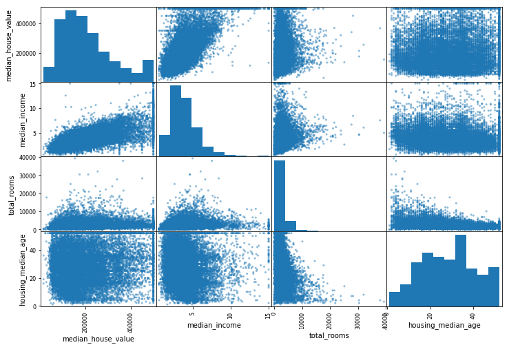
分析:
- 对角线部分: 核密度估计图(Kernel Density Estimation),就是用来看某 一个 变量分布情况,横轴对应着该变量的值,纵轴对应着该变量的密度(可以理解为出现频次)。
- 非对角线部分:两个变量之间分布的关联散点图。将任意两个变量进行配对,以其中一个为横坐标,另一个为纵坐标,将所有的数据点绘制在图上,用来衡量两个变量的关联度(Correlation)。
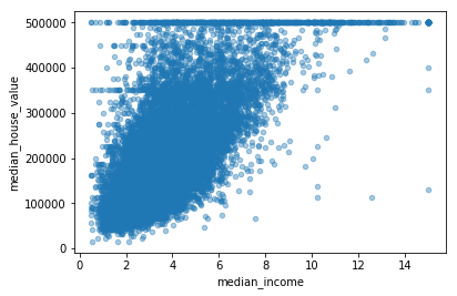
# 放大关联性最大的图
housing.plot(kind="scatter", x="median_income",
             y="median_house_value", alpha=0.4)
plt.show()
5.为算法准备数据
5.1 数据清理
5.11取出标签值“median_house_vlaue” -->因为这个是预测值
housing = housing.drop("median_house_value", axis=1)
housing_label = strat_train_set["median_house_value"].copy()
5.12 数据清洗
数据清洗一般有两种策略,一种是直接丢弃不用的数据,第二个是将不好的数据置零/平均数/中位数
下面有3中选择:
- 选择 1 ->丢弃相应的数据
- 选择 2 ->丢弃这个属性
- 选择 3 ->用特殊的数据填补
housing.dropna(subset=["total_bedrooms"])  # subset指定某列进行dropna(数据清洗)
housing.drop("total_bedrooms", axis=1)
median = housing["total_bedrooms"].median()
housing["total_bedrooms"].fillna(median)
17606     351.0
18632     108.0
14650     471.0
3230      371.0
3555     1525.0
19480     588.0
8879      317.0
13685     293.0
4937      465.0
4861      229.0
16365     951.0
19684     559.0
19234     501.0
13956     582.0
2390      495.0
11176     649.0
15614     545.0
2953      251.0
13209     409.0
6569      261.0
5825      913.0
18086     538.0
16718     945.0
13600     278.0
13989     444.0
15168     190.0
6747      563.0
7398      366.0
5562      133.0
16121     416.0
          ...
12380     767.0
5618       24.0
10060     539.0
18067     438.0
4471      797.0
19786     300.0
9969      393.0
14621    1051.0
579       302.0
11682    1615.0
245       460.0
12130     537.0
16441     544.0
11016     428.0
19934     422.0
1364       34.0
1236      829.0
5364      272.0
11703     300.0
10356     449.0
15270     515.0
3754      373.0
12166     756.0
6003      932.0
7364      212.0
6563      236.0
12053     294.0
13908     872.0
11159     380.0
15775     682.0
Name: total_bedrooms, Length: 16512, dtype: float64
5.13使用sk-learn对缺失值处理
from sklearn.impute import SimpleImputer
# 创建Imputer实例,使用median处理缺失数据-->创建一种策略
imputer = SimpleImputer(strategy="median")
# imputer只能处理数值属性,所以先删除Ocean属性
housing_num = housing.drop("ocean_proximity", axis=1)
# fit将inputer适配到数据集,这里会计算所有保留属性的中位数,保存在变量statistics中
imputer.fit(housing_num)
print(imputer.statistics_)
print(housing_num.median().values)
# 替换缺失值,返回一个Pandas DataFrame数组。
X = imputer.transform(housing_num)
# 将DataFrame存到housing_tr中
housing_tr = pd.DataFrame(X, columns=housing_num.columns)
[-1.18510000e+02  3.42600000e+01  2.90000000e+01  2.11950000e+03
  4.33000000e+02  1.16400000e+03  4.08000000e+02  3.54090000e+00
  5.23228423e+00  2.03031374e-01  2.81765270e+00]
[-1.18510000e+02  3.42600000e+01  2.90000000e+01  2.11950000e+03
  4.33000000e+02  1.16400000e+03  4.08000000e+02  3.54090000e+00
  5.23228423e+00  2.03031374e-01  2.81765270e+00]
5.2 处理文本和分类属性
5.21 使用转换器将ocean属性的文本属性转化为数值属性
from sklearn.preprocessing import LabelEncoder
encode = LabelEncoder()  # 创建转换器对象
housing_cat = housing["ocean_proximity"]
housing_cat_encoded = encode.fit_transform(housing_cat)  # 使用转换器转换
# print(housing_cat_encoded)
# print(encode.classes_)  # 其实转换器的使用和清洗器imputer是一样的,sklearn内部api具有很强的一致性
- 使用数据转换之后会发现,原本ocean里面的文本数据只是用来标记类别的,转换器转换之后,类别之间有了大小的关系而这样的大小关系是没有需要的,所以单纯用1234等来标记类别通常是不合理的。分类器做分类时,往往会认为这样的数据是连续并且有序的,用012345来表示各个类别之间关系与原来的关系不一样了。所以这里可以使用独热编码
#   使用独热编码
from sklearn.preprocessing import OneHotEncoder

encode = OneHotEncoder(categories='auto')
# housing_cat_1hout是一个稀疏矩阵
housing_cat_1hot = encode.fit_transform(housing_cat_encoded.reshape(-1, 1))
print(housing_cat_1hot.toarray())             # 稀疏矩阵转化为Numpy数组
[[1. 0. 0. 0. 0.]
 [1. 0. 0. 0. 0.]
 [0. 0. 0. 0. 1.]
 ...
 [0. 1. 0. 0. 0.]
 [1. 0. 0. 0. 0.]
 [0. 0. 0. 1. 0.]]
#  sklearn里面其他的转换方法LabelBinarizer(一次性从文本变成数字及oneHot编码)
from sklearn.preprocessing import LabelBinarizer
encode = LabelBinarizer()  # 如果加参数sparse_output=True下面返回的就是稀疏矩阵
housing_cat_1hot = encode.fit_transform(
    housing_cat)                       # 直接是Numpy类型
print(housing_cat_1hot)
[[1 0 0 0 0]
 [1 0 0 0 0]
 [0 0 0 0 1]
 ...
 [0 1 0 0 0]
 [1 0 0 0 0]
 [0 0 0 1 0]]
5.22 自定义转换器
对下面代码的理解:
- 首先,按照数据的范围设置界限分别来取room bedroom population以及household的值
然后,attr_adder初始化,调用类初始化,设置要不要每个房子的卧室数目。调用transform函数
对数据进行处理,然后使用np.c_函数进行合并 np.c_是列合并,要求列数一致, np.r_是行合并。 - 在本例中,转换器有一个超参数add_bedrooms_per_room默认设
置为True(提供合理的默认值通常是很有帮助的)。这个超参数可以
让你轻松知晓添加这个属性是否有助于机器学习的算法。更广泛地
说,如果你对数据准备的步骤没有充分的信心,就可以添加这个超参
数来进行把关。这些数据准备步骤的执行越自动化,你自动尝试的
组合也就越多,从而有更大可能从中找到一个重要的组合(还节省了大
量时间)。
from sklearn.base import BaseEstimator, TransformerMixin
rooms_ix, bedrooms_ix, population_ix, household_ix = 3, 4, 5, 6


class CombineAttributesAdder(BaseEstimator, TransformerMixin):
    def __init__(self, add_bedrooms_per_room=True):
        self.add_bedrooms_per_room = add_bedrooms_per_room

    def fit(self, X, y=None):
        return self

    def transform(self, X, y=None):
        rooms_per_household = X[:, rooms_ix]/X[:, household_ix]
        population_per_household = X[:, population_ix]/X[:, household_ix]
        if self.add_bedrooms_per_room:
            bedrooms_per_room = X[:, bedrooms_ix]/X[:, rooms_ix]
            return np.c_[X, rooms_per_household, population_per_household, bedrooms_per_room]
        else:
            return np.c_[X, rooms_per_household, population_per_household]


attr_adder = CombineAttributesAdder(add_bedrooms_per_room=False)
housing_extra_arrtibs = attr_adder.transform(housing.values)
print(housing_extra_arrtibs)
[[-121.89 37.29 38.0 ... 2.094395280235988 4.625368731563422
  2.094395280235988]
 [-121.93 37.05 14.0 ... 2.7079646017699117 6.008849557522124
  2.7079646017699117]
 [-117.2 32.77 31.0 ... 2.0259740259740258 4.225108225108225
  2.0259740259740258]
 ...
 [-116.4 34.09 9.0 ... 2.742483660130719 6.34640522875817
  2.742483660130719]
 [-118.01 33.82 31.0 ... 3.808988764044944 5.50561797752809
  3.808988764044944]
 [-122.45 37.77 52.0 ... 1.9859154929577465 4.843505477308295
  1.9859154929577465]]
5.3 特征缩放
分析:
- 特征缩放常用于输入的数值属性有很大的比例差异的时候,因为这种差异往往会导致算法性能下降。
当然也有特例,具体问题具体分析。在这个例子里面,地区房间的总数在(6,39320)之间,
而收入的中位数在(0-15)之间,所以需要特征缩放。 - 特征缩放常用的两种方法:(两种估算器)
- 最小最大缩放
最大最小缩放又叫归一化,目的是将值的范围缩小到0-1之间。(不一定要是0-1)
实现方法是将值减去min并除以(max-min)。
在sklearn中的实现是MinMaxScaler方法,可以使用feature_range修改(0-1)的范围。 - 标准化
标准化是用当前值减去平均值再除以反差,让结果分布具备单位方差。
标准化没有固定的范围,其特点是受异常值的影响更小。
在sklearn中的实现是StandadScaler方法。
- 最小最大缩放
5.4 使用流水线转换数据
5.41流水线示例:
- 缺失值处理-> 合并新属性->标准化(结构:转换器-转换器-估算器,除最后一个外必须是转换器)
- 调用方法:当流水线调用fit_transform方法时,对于前两个转换器,会先调用fit()方法,直到到转换器,到转换器调用transform方法。 所以对于这种流水线直接调用fit_transform即可。
from sklearn.pipeline import Pipeline
from sklearn.preprocessing import StandardScaler
from sklearn.base import BaseEstimator, TransformerMixin
# Scikit-Learn中没有可以用来处理Pandas DataFrames的,因此我们需要为此任务编写一个简单的自定义转换器:


class DataFrameSelector(BaseEstimator, TransformerMixin):
    def __init__(self, attribute_names):
        self.attribute_names = attribute_names

    def fit(self, X, y=None):
        return self

    def transform(self, X):
        return X[self.attribute_names].values


num_pipline = Pipeline([
    ('Simpleimputer', SimpleImputer(strategy="median")),
    ('attribs_adder', CombineAttributesAdder()),
    ('std_scaler', StandardScaler()),
])
housing_num_str = num_pipline.fit_transform(housing_num)
print("-"*30)
print(housing_num_str)
------------------------------
[[-1.15604281  0.77194962  0.74333089 ... -0.31205452 -0.08649871
   0.15531753]
 [-1.17602483  0.6596948  -1.1653172  ...  0.21768338 -0.03353391
  -0.83628902]
 [ 1.18684903 -1.34218285  0.18664186 ... -0.46531516 -0.09240499
   0.4222004 ]
 ...
 [ 1.58648943 -0.72478134 -1.56295222 ...  0.3469342  -0.03055414
  -0.52177644]
 [ 0.78221312 -0.85106801  0.18664186 ...  0.02499488  0.06150916
  -0.30340741]
 [-1.43579109  0.99645926  1.85670895 ... -0.22852947 -0.09586294
   0.10180567]]
5.42完整的流水线处理
- 完整的流水线处理包含了缺失值处理-> 合并新属性->标准化->字符数据独热编码
- 下面的selector是数据选择
- sklearn 的FeatureUnion类最终可以合并所有流水线的所产生的数据
from sklearn.pipeline import FeatureUnion
from sklearn_features.transformers import DataFrameSelector


num_attribs = list(housing_num)
cat_attribs = ["ocean_proximity"]
# 第一条流水线
num_pipeline = Pipeline([
    ('selector', DataFrameSelector(num_attribs)),
    ('Simpleimputer', SimpleImputer(strategy="median")),
    ('attribs_adder', CombineAttributesAdder()),
    ('std_scaler', StandardScaler()),
])
# 第二条流水线
# cat_pipeline = Pipeline([
#     ('selector',DataFrameSelector(cat_attribs)),
#     ('label_binarizer',LabelBinarizer()),
# ])
# * 这里书上的代码旧了,sklearn0.19重写了fit_tansforms,新的trans_form只接收两个参数,
# 流水线执行LabelBinarizer会传入3个参数,重写一个LabelBinarizer方法
from sklearn.base import TransformerMixin


class MyLabelBinarizer(TransformerMixin):
    def __init__(self, *args, **kwargs):
        self.encoder = LabelBinarizer(*args, **kwargs)

    def fit(self, x, y=0):
        self.encoder.fit(x)
        return self

    def transform(self, x, y=0):
        return self.encoder.transform(x)


cat_pipeline = Pipeline([
    ('selector', DataFrameSelector(cat_attribs)),
    ('label_binarizer', MyLabelBinarizer()),
])
# 合并流水线
full_pipeline = FeatureUnion(transformer_list=[
    ("num_pipline", num_pipeline),
    ("cat_pipline", cat_pipeline),
])
# 运行流水线
housing_prepared = full_pipeline.fit_transform(housing)
print(housing_prepared)
print(housing_prepared.shape)
[[-1.15604281  0.77194962  0.74333089 ...  0.          0.
   0.        ]
 [-1.17602483  0.6596948  -1.1653172  ...  0.          0.
   0.        ]
 [ 1.18684903 -1.34218285  0.18664186 ...  0.          0.
   1.        ]
 ...
 [ 1.58648943 -0.72478134 -1.56295222 ...  0.          0.
   0.        ]
 [ 0.78221312 -0.85106801  0.18664186 ...  0.          0.
   0.        ]
 [-1.43579109  0.99645926  1.85670895 ...  0.          1.
   0.        ]]
(16512, 19)
6 模型选择和训练
6.1 训练训练集
- 线性回归模型:LR
from sklearn.linear_model import LinearRegression

lin_reg = LinearRegression()
lin_reg.fit(housing_prepared, housing_label)
# 取前5行
some_data = housing.iloc[:5]
some_labels = housing_label.iloc[:5]
some_data_prepared = full_pipeline.transform(some_data)
print("Predictions:\t", lin_reg.predict(some_data_prepared))
print("Labels:\t\t", list(some_labels))
print(lin_reg.intercept_)
print(lin_reg.coef_)
Predictions:     [209420.50610494 315409.32621299 210124.77314125  55983.75406116
 183462.63421725]
Labels:      [286600.0, 340600.0, 196900.0, 46300.0, 254500.0]
235473.80836449962
[-56129.06165758 -56723.67757798  13971.77259524   7327.89108513
   2200.80894803 -45937.59348295  41468.93537123  78337.91915705
   3575.6306461   19109.54513283    447.54395435   3575.6306461
    447.54395435  -2825.3656443  -17506.92104904 -51684.61814988
 105578.16342067 -22242.22267579 -14144.40154595]
# 对线性回归模型执行交叉验证
from sklearn.model_selection import cross_val_score
lin_score = cross_val_score(lin_reg, housing_prepared,
                            housing_label, scoring="neg_mean_squared_error", cv=10)
lin_rmse_score = np.sqrt(-lin_score)
print(lin_rmse_score)
print("Mean:", lin_rmse_score.mean())
print("Standard deviation:", lin_rmse_score.std())
[66062.46546015 66793.78724541 67644.87711878 74702.95282053
 68054.75502851 70902.35184092 64171.47270772 68081.38734615
 71042.4918974  67281.01437174]
Mean: 68473.75558372994
Standard deviation: 2844.0256903763307
6.2 均方误差
- 到此,预测已经结束,但是观察上面的Prediction和Labels的大小,还有很大的误差。
下面使用均方误差来评估和调整模型。
from sklearn.metrics import mean_squared_error
housing_predictions = lin_reg.predict(housing_prepared)
lin_mse = mean_squared_error(housing_label, housing_predictions)
lin_rmse = np.sqrt(lin_mse)
print(lin_rmse)
68147.95744947501
6.3 决策树模型DTR
- LR的均方误差很大,拟合不够。 所以换一个模型测试一下。
# * LR的均方误差很大,拟合不够。 所以换一个模型测试一下。
from sklearn.tree import DecisionTreeRegressor

tree_reg = DecisionTreeRegressor()
tree_reg.fit(housing_prepared, housing_label)
housing_predictions = tree_reg.predict(housing_prepared)
tree_mse = mean_squared_error(housing_label, housing_predictions)
tree_rmse = np.sqrt(tree_mse)
print(tree_rmse)
0.0
6.4 交叉验证
- 使用决策树模型发现误差为0,这代表肯定过拟合了。
- 下面使用交叉验证来更好的评估决策树模型。
from sklearn.model_selection import cross_val_score
# 十折交叉验证
score = cross_val_score(tree_reg, housing_prepared,
                        housing_label, scoring="neg_mean_squared_error", cv=10)
rmse_score = np.sqrt(-score)
print(rmse_score)
print("Mean:", rmse_score.mean())
print("Standard deviation:", rmse_score.std())
# 这里的输出指:交叉验证决策树获得的分数是rmse_score.mean(),上下浮动rmse_score.std()个数值。
[70190.39079163 66064.66678933 70919.2241942  69755.78097769
 71539.03243522 74039.67372515 70437.47726481 70239.92318825
 75076.56450274 69247.65253169]
Mean: 70751.0386400731
Standard deviation: 2367.7244306133935
6.5 随机森林
# 上面两个模型都不尽如人意,所以测试第三个模型:RF
from sklearn.ensemble import RandomForestRegressor
forest_reg = RandomForestRegressor()
forest_reg.fit(housing_prepared, housing_label)
housing_predictions = forest_reg.predict(housing_prepared)
score = cross_val_score(forest_reg, housing_prepared,
                        housing_label, scoring="neg_mean_squared_error", cv=10)
forest_rmse_score = np.sqrt(-score)
print(forest_rmse_score)
print("Mean:", forest_rmse_score.mean())
print("Standard deviation:", forest_rmse_score.std())

print("Predictions:\t", forest_reg.predict(some_data_prepared))  # 预测样本
print("Labels:\t\t", list(some_labels))         # 实际值
D:\Anaconda3\lib\site-packages\sklearn\ensemble\forest.py:248: FutureWarning: The default value of n_estimators will change from 10 in version 0.20 to 100 in 0.22.
  "10 in version 0.20 to 100 in 0.22.", FutureWarning)
[52198.48245471 49190.66608383 52933.46838462 55013.84784886
 51547.27239792 56007.14126735 51188.89643343 51095.69872494
 55675.80059914 51441.22938544]
Mean: 52629.25035802469
Standard deviation: 2132.8000877264612
Predictions:     [261400. 327800. 247480.  46540. 238250.]
Labels:      [286600.0, 340600.0, 196900.0, 46300.0, 254500.0]
6.6 模型保存
- 训练好的模型要进行保存,相关结果也要进行保存。
- 使用python的pickel模块或sklearn.externals.joblib模块保存模型。
from sklearn.externals import joblib
joblib.dump(forest_reg, "my_model.pkl")         # 保存
my_model_loaded = joblib.load("my_model.pkl")  # 导入V
7.模型优化
7.1 网格搜索
- 除了手动操作调整超参数,还可以通过算法自动调整超参数,第一个就是网格搜索方法(GridSearchCV)
网格搜索是一种穷举的搜索方案,即将所有参数的所有可能的组合组成一个表格,对各个参数逐一计算。
网格搜索的结果好坏与数据集的划分有很大的关系,所以网格搜索常常与交叉验证一起使用。
Grid Search调参方法存在的弊端是参数越多,候选值越多,耗费时间越长。所以,一般情况下,先定一个大范围,然后再细化。
from sklearn.model_selection import GridSearchCV
para_grid = [
    {'n_estimators':[3,10,30],'max_features':[2,4,6,8]},   # 3*4网格搜索,12种
    {'bootstrap':[False],'n_estimators':[3,10],'max_features':[2,3,4]} # 2*3 6种 共18种组合
]
forest_reg2 = RandomForestRegressor()
# 配合五折交叉搜索,18*5 = 90 次,总共进行了90次的模型训练
grid_search = GridSearchCV(forest_reg2,para_grid,cv=5,scoring="neg_mean_squared_error")
grid_search.fit(housing_prepared,housing_label)
print(grid_search.best_params_)  # 打印最佳参数
print(grid_search.best_estimator_) # 最佳模型
cvres = grid_search.cv_results_     # 评估分数
for mean_score,params in zip(cvres["mean_test_score"],cvres["params"]):
    print(np.sqrt(-mean_score),params)
{'max_features': 8, 'n_estimators': 30}
RandomForestRegressor(bootstrap=True, criterion='mse', max_depth=None,
           max_features=8, max_leaf_nodes=None, min_impurity_decrease=0.0,
           min_impurity_split=None, min_samples_leaf=1,
           min_samples_split=2, min_weight_fraction_leaf=0.0,
           n_estimators=30, n_jobs=None, oob_score=False,
           random_state=None, verbose=0, warm_start=False)
64284.877079430145 {'max_features': 2, 'n_estimators': 3}
56787.08219950486 {'max_features': 2, 'n_estimators': 10}
54634.8597925206 {'max_features': 2, 'n_estimators': 30}
62625.13023634532 {'max_features': 4, 'n_estimators': 3}
54178.71450231148 {'max_features': 4, 'n_estimators': 10}
52166.9297650929 {'max_features': 4, 'n_estimators': 30}
60632.06160053902 {'max_features': 6, 'n_estimators': 3}
53671.382898481956 {'max_features': 6, 'n_estimators': 10}
51209.764682060915 {'max_features': 6, 'n_estimators': 30}
60205.08228898087 {'max_features': 8, 'n_estimators': 3}
53046.02597867227 {'max_features': 8, 'n_estimators': 10}
50988.49917680898 {'max_features': 8, 'n_estimators': 30}
64237.4676969949 {'bootstrap': False, 'max_features': 2, 'n_estimators': 3}
55863.58989745313 {'bootstrap': False, 'max_features': 2, 'n_estimators': 10}
61235.68857900436 {'bootstrap': False, 'max_features': 3, 'n_estimators': 3}
54690.58049493668 {'bootstrap': False, 'max_features': 3, 'n_estimators': 10}
59267.34518636521 {'bootstrap': False, 'max_features': 4, 'n_estimators': 3}
53190.09578420519 {'bootstrap': False, 'max_features': 4, 'n_estimators': 10}
7.2 随机搜索
- 当需要搜索的组合很多时,就不适合使用表格搜索了。此时通常使用随机搜索(RandomizedSearchCV)
随机搜索不会穷尽所有参数,它会在参数空间随机采样。 - 随机搜索策略:
- 对于搜索范围是distribution的超参数,根据给定的distribution随机采样;
- 对于搜索范围是list的超参数,在给定的list中等概率采样;
- 对a、b两步中得到的n_iter组采样结果,进行遍历。
- (补充)如果给定的搜索范围均为list,则不放回抽样n_iter次。
- 随机搜索的优点:
如果运行随机搜索1000个迭代,那么将会探索每个超参数的1000个不同的值(而不是像网格搜索方法那样每个超参数仅探索少量几个值)。
通过简单地设置迭代次数,可以更好地控制要分配给探索的超参数的计算预算。
7.3 集成方法
还有一种调整方法就是将各个好的模型集成起来,组合成一个集成模型。(类似随机森林)
7.4 模型分析
from sklearn.preprocessing import LabelEncoder
feature_importances=grid_search.best_estimator_.feature_importances_
print(feature_importances)
encoder=LabelEncoder()
housing_cat=housing["ocean_proximity"]
housing_cat_encoded=encoder.fit_transform(housing_cat)
extra_attribs=["rooms_per_household","pop_per_household","bedrooms_per_room"]
cat_one_hot_attribs=list(encoder.classes_)
attribus=num_attribs+extra_attribs+cat_one_hot_attribs
sorted(zip(feature_importances,attribus),reverse=True)
[6.49886314e-02 5.75244728e-02 3.99323296e-02 1.34508217e-02
 1.30533240e-02 1.29077646e-02 1.32840680e-02 3.34406458e-01
 3.95819895e-02 5.44151119e-02 6.77111178e-02 2.95775829e-02
 5.97611143e-02 2.87285632e-02 8.84117371e-03 1.54870133e-01
 1.39273664e-04 3.15616780e-03 3.66990154e-03]
[(0.3344064582565652, 'median_income'),
 (0.1548701334803861, 'INLAND'),
 (0.06771111779862625, 'population_per_household'),
 (0.06498863136588338, 'longitude'),
 (0.059761114331979774, 'pop_per_household'),
 (0.05752447280722709, 'latitude'),
 (0.05441511192586514, 'bedrooms_per_house'),
 (0.039932329606253154, 'housing_median_age'),
 (0.03958198945470592, 'room_per_household'),
 (0.02957758287533781, 'rooms_per_household'),
 (0.028728563174464258, 'bedrooms_per_room'),
 (0.013450821682219134, 'total_rooms'),
 (0.013284067951082463, 'households'),
 (0.013053323968912556, 'total_bedrooms'),
 (0.012907764611245971, 'population'),
 (0.008841173709972056, '<1H OCEAN'),
 (0.003669901537931307, 'NEAR OCEAN'),
 (0.0031561677969219157, 'NEAR BAY'),
 (0.00013927366442045662, 'ISLAND')]
8. 测试模型
final_model = grid_search.best_estimator_

x_test = strat_test_set.drop("median_house_value",axis=1)
y_test = strat_test_set["median_house_value"].copy()
x_test_prepared = full_pipeline.transform(x_test)
final_predications = final_model.predict(x_test_prepared)
final_mse = mean_squared_error(y_test,final_predications)
final_rmse = np.sqrt(final_mse)
print(final_rmse)
48557.63204741025
8.1 计算95%的置信区间
from scipy import stats
confidence = 0.95
squared_errors = (final_predications-y_test)**2  # 平方误差
mean = squared_errors.mean()
m = len(squared_errors)

confidence_interval = np.sqrt(stats.t.interval(confidence, m-1, loc=np.mean(squared_errors),
                                               scale=stats.sem(squared_errors)))
print(confidence_interval)
9. 课后练习
9.1 课后练习1:SVR预测器
使用网格搜索寻找SVR预测器中最好的参数
from sklearn.model_selection import GridSearchCV
from sklearn.svm import SVR
para_grid = [
    {'kernel':['linear'],'C':[10.,30.,100.,300.,1000.,3000.,10000.,30000.0]},
    {'kernel':['rbf'],'C':[1.0,3.0,10.,30.,100.,300.,1000.0],
    'gamma':[0.01,0.03,0.1,0.3,1.0,3.0]},
]                                                       # 参数列表
svm_reg = SVR()
grid_search = GridSearchCV(svm_reg,para_grid,cv=5,scoring = 'neg_mean_squared_error',verbose = 2,n_jobs=4)
grid_search.fit(housing_prepared,housing_label)
negative_mse = grid_search.best_score_
rmse = np.sqrt(-negative_mse)
print(rmse)
print(grid_search.best_params_)
9.2 课后练习2:替换随机搜索调参方法
from sklearn.model_selection import RandomizedSearchCV
from scipy.stats import expon, reciprocal
param_distribs = {
        'kernel': ['linear', 'rbf'],
        'C': reciprocal(20, 200000),
        'gamma': expon(scale=1.0),
    }

svm_reg = SVR()
rnd_search = RandomizedSearchCV(svm_reg, param_distributions=param_distribs,
                                n_iter=50, cv=5, scoring='neg_mean_squared_error',
                                verbose=2, n_jobs=4, random_state=42)
rnd_search.fit(housing_prepared, housing_label)
negative_mse = rnd_search.best_score_
rmse = np.sqrr(-negative_mse)
print(rmse)