猫和狗分类器---降低过拟合

猫与狗图像分类

练习2：减少过度拟合

预计完成时间：30分钟

在这个笔记本中，我们将基于我们在练习1中创建的模型来对猫与狗进行分类，并通过采用一些策略来减少过度拟合来提高准确性：数据增加和退出。

我们将遵循以下步骤：

1.通过对训练图像进行随机变换来探索数据增强的工作原理。
2.将数据扩充添加到我们的数据预处理中。
3.将退出添加到预定。
4.重新训练模型并评估损失和准确性。

让我们开始吧！

探索数据扩充

让我们熟悉数据增强的概念，这是对抗计算机视觉模型过度拟合的重要方法。

为了充分利用我们的一些训练样例，我们将通过一系列随机变换“增强”它们，这样在训练时，我们的模型将永远不会看到完全相同的两次图片。这有助于防止过度拟合，并有助于模型更好地概括。

这可以通过配置要对我们的`ImageDataGenerator实例读取的图像执行的多个随机转换来完成。让我们开始一个例子：

from tensorflow.keras.preprocessing.image import ImageDataGenerator

datagen = ImageDataGenerator(
      rotation_range=40,
      width_shift_range=0.2,
      height_shift_range=0.2,
      shear_range=0.2,
      zoom_range=0.2,
      horizontal_flip=True,
      fill_mode='nearest')

这些只是一些可用的选项（更多信息，请参阅[Keras文档]（https://keras.io/preprocessing/image/）。让我们快速浏览一下我们刚写的内容：

• rotation_range是一个度数（0-180）的值，一个随机旋转图片的范围。
• width_shift和height_shift是范围（作为总宽度或高度的一部分），在其中垂直或水平地随机翻译图片。
• shear_range用于随机应用剪切变换。
• zoom_range用于随机缩放图片内部。
• horizo​​ntal_flip用于水平随机翻转一半图像。当没有水平不对称假设（例如真实世界的图片）时，这是相关的。
• fill_mode是用于填充新创建的像素的策略，可以在旋转或宽度/高度偏移后出现。

我们来看看我们的增强图像。首先让我们设置我们的示例文件，如练习1中所示。
注意：本练习中使用的2,000张图片摘自Kaggle提供的[“Dogs vs. Cats”数据集]（https://www.kaggle.com/c/dogs-vs-cats/data） ，其中包含25,000张图片。在这里，我们使用完整数据集的子集来减少用于教育目的的培训时间。

!wget --no-check-certificate \
   https://storage.googleapis.com/mledu-datasets/cats_and_dogs_filtered.zip -O \
   /tmp/cats_and_dogs_filtered.zip

import os
import zipfile

local_zip = '/tmp/cats_and_dogs_filtered.zip'
zip_ref = zipfile.ZipFile(local_zip, 'r')
zip_ref.extractall('/tmp')
zip_ref.close()
  
base_dir = '/tmp/cats_and_dogs_filtered'
train_dir = os.path.join(base_dir, 'train')
validation_dir = os.path.join(base_dir, 'validation')

# Directory with our training cat pictures
train_cats_dir = os.path.join(train_dir, 'cats')

# Directory with our training dog pictures
train_dogs_dir = os.path.join(train_dir, 'dogs')

# Directory with our validation cat pictures
validation_cats_dir = os.path.join(validation_dir, 'cats')

# Directory with our validation dog pictures
validation_dogs_dir = os.path.join(validation_dir, 'dogs')

train_cat_fnames = os.listdir(train_cats_dir)
train_dog_fnames = os.listdir(train_dogs_dir)

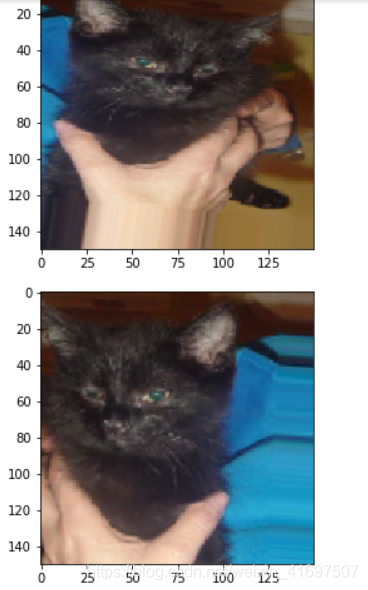
接下来，让我们将datagen转换应用于训练集中的猫图像，以生成五个随机变体。 重新运行细胞几次以查看新批次的随机变体。

%matplotlib inline

import matplotlib.pyplot as plt
import matplotlib.image as mpimg

from tensorflow.keras.preprocessing.image import array_to_img, img_to_array, load_img

img_path = os.path.join(train_cats_dir, train_cat_fnames[2])
img = load_img(img_path, target_size=(150, 150))  # this is a PIL image
x = img_to_array(img)  # Numpy array with shape (150, 150, 3)
x = x.reshape((1,) + x.shape)  # Numpy array with shape (1, 150, 150, 3)

# The .flow() command below generates batches of randomly transformed images
# It will loop indefinitely, so we need to `break` the loop at some point!
i = 0
for batch in datagen.flow(x, batch_size=1):
  plt.figure(i)
  imgplot = plt.imshow(array_to_img(batch[0]))
  i += 1
  if i % 5 == 0:
    break

将数据扩充添加到预处理步骤

现在让我们将[Exploring Data Augmentation]（＃scrollTo = E3sSwzshfSpE）的数据增强转换添加到我们的数据预处理配置中：

# Adding rescale, rotation_range, width_shift_range, height_shift_range,
# shear_range, zoom_range, and horizontal flip to our ImageDataGenerator
train_datagen = ImageDataGenerator(
    rescale=1./255,
    rotation_range=40,
    width_shift_range=0.2,
    height_shift_range=0.2,
    shear_range=0.2,
    zoom_range=0.2,
    horizontal_flip=True,)

# Note that the validation data should not be augmented!
test_datagen = ImageDataGenerator(rescale=1./255)

# Flow training images in batches of 32 using train_datagen generator
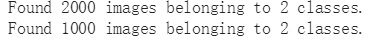
train_generator = train_datagen.flow_from_directory(
        train_dir,  # This is the source directory for training images
        target_size=(150, 150),  # All images will be resized to 150x150
        batch_size=20,
        # Since we use binary_crossentropy loss, we need binary labels
        class_mode='binary')

# Flow validation images in batches of 32 using test_datagen generator
validation_generator = test_datagen.flow_from_directory(
        validation_dir,
        target_size=(150, 150),
        batch_size=20,
        class_mode='binary')

如果我们使用此数据增强配置训练新网络，我们的网络将永远不会看到相同的输入两次。 然而，它看到的输入仍然是非常相互关联的，所以这可能不足以完全摆脱过度拟合。

添加Dropout

另一种对抗过度拟合的流行策略是使用Dropout。
提示：要了解有关辍学的更多信息，请参阅[机器中的[培训神经网络]（https://developers.google.com/machine-learning/crash-course/training-neural-networks/video-lecture） 学习速成课程]（https://developers.google.com/machine-learning/crash-course/）。[链接文字]（HTTPS：//）
让我们从练习1重新配置我们的convnet架构，在最终分类层之前添加一些丢失：

from tensorflow.keras import layers
from tensorflow.keras import Model
from tensorflow.keras.optimizers import RMSprop

# Our input feature map is 150x150x3: 150x150 for the image pixels, and 3 for
# the three color channels: R, G, and B
img_input = layers.Input(shape=(150, 150, 3))

# First convolution extracts 16 filters that are 3x3
# Convolution is followed by max-pooling layer with a 2x2 window
x = layers.Conv2D(16, 3, activation='relu')(img_input)
x = layers.MaxPooling2D(2)(x)

# Second convolution extracts 32 filters that are 3x3
# Convolution is followed by max-pooling layer with a 2x2 window
x = layers.Conv2D(32, 3, activation='relu')(x)
x = layers.MaxPooling2D(2)(x)

# Third convolution extracts 64 filters that are 3x3
# Convolution is followed by max-pooling layer with a 2x2 window
x = layers.Convolution2D(64, 3, activation='relu')(x)
x = layers.MaxPooling2D(2)(x)

# Flatten feature map to a 1-dim tensor
x = layers.Flatten()(x)

# Create a fully connected layer with ReLU activation and 512 hidden units
x = layers.Dense(512, activation='relu')(x)

# Add a dropout rate of 0.5
x = layers.Dropout(0.5)(x)

# Create output layer with a single node and sigmoid activation
output = layers.Dense(1, activation='sigmoid')(x)

# Configure and compile the model
model = Model(img_input, output)
model.compile(loss='binary_crossentropy',
              optimizer=RMSprop(lr=0.001),
              metrics=['acc'])

重新训练模型

随着数据增加和退出，让我们重新培训我们的convnet模型。 这一次，让我们训练所有2000个可用图像，包括30个时期，并对所有1,000个测试图像进行验证。 （这可能需要几分钟才能运行。）看看你是否可以自己编写代码：

# WRITE CODE TO TRAIN THE MODEL ON ALL 2000 IMAGES FOR 30 EPOCHS, AND VALIDATE 
# ON ALL 1,000 TEST IMAGES

解决方案

单击下面的解决方案。

history = model.fit_generator(
      train_generator,
      steps_per_epoch=100,
      epochs=30,
      validation_data=validation_generator,
      validation_steps=50,
      verbose=2)

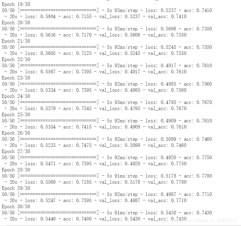
请注意，在数据增加到位的情况下，每次新的训练时期运行时，2,000个训练图像都会随机变换，这意味着模型在训练期间将永远不会看到相同的图像两次。

评估结果

让我们用数据增加和退出来评估模型训练的结果：

# Retrieve a list of accuracy results on training and test data
# sets for each training epoch
acc = history.history['acc']
val_acc = history.history['val_acc']

# Retrieve a list of list results on training and test data
# sets for each training epoch
loss = history.history['loss']
val_loss = history.history['val_loss']

# Get number of epochs
epochs = range(len(acc))

# Plot training and validation accuracy per epoch
plt.plot(epochs, acc)
plt.plot(epochs, val_acc)
plt.title('Training and validation accuracy')

plt.figure()

# Plot training and validation loss per epoch
plt.plot(epochs, loss)
plt.plot(epochs, val_loss)
plt.title('Training and validation loss')

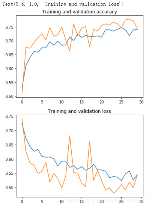
好多了！ 我们不再过度拟合，我们已经获得了大约3个验证准确率百分点（参见顶部图表中的绿线）。 事实上，根据我们的培训资料，我们可以保持我们的模型超过30多个时代，我们可能达到~80％！

清理

在运行下一个练习之前，运行以下单元格以终止内核并释放内存资源：

import os, signal
os.kill(os.getpid(), signal.SIGKILL)