一、逻辑回归介绍
回归一般用于解决那些连续变量的问题,如:线性回归,它是通过最小化误差函数,来不断拟合一条直线,以计算出权重w和偏差 b的过程,它的目标是基于一个连续方程去预测一个值。 逻辑回归(Logistic Regression)是机器学习中的一种分类模型。
1、Logistic 函数的逆函数 –> Logit 函数
在了解 Logistic 函数之前,我们先来了解一下它的逆函数 Logit 函数,即对数几率函数。正如我们所了解的一样逆函数之间关于 y = x 直线对称,自变量 x 和因变量 y 互为对偶位置,因此,Logit 函数和 Logistic 函数有很多性质都有关联。
Logit 函数的变量需要一个概率值 p 作为自变量,如果是二分类问题,确切一点是伯努利分布(即二项分布),如果是多分类问题,则是多项分布。
2、伯努利分布
它又称为二项分布,也就是说它只能表示成功和失败两种情况。当是二分类问题时,都可用该分布
取 1,表示成功,以概率 p 表示
取 0,即失败,以概率 q = 1-p 表示
伯努利分布的概率函数可以表示为: Pr(X=1) = 1 - Pr(X=0) = 1-q = p
此外,Logistic 函数也是属于广义线性模型(GLM)的一种,在建立广义线性模型之前,我们还需要从线性函数开始,从独立的连续变量映射到一个概率分布。
而如果是针对二分类的 Logistic 回归,由于是二分类属于二值选项问题,我们一般会将上面的概率分布建模成一个伯努利分布(即二项分布),而将上述的独立的连续变量建模成线性方程回归后的 y 值,最后再通过连接函数,这里采用对数几率函数 Ligit ,将连续的 y = wx +b 的线性连续变量映射到二项分布。
只是,我们先将 Logit 函数,它的映射是从自变量 p(即二项分布发生的几率) 到 函数值(即y=wx+b,也就是连接函数y即 logit(p)) 的映射,故逆函数 Logistic 函数即上一段所讲,便可以将连续值映射到二项分布,从而用做分类问题。
3、logits函数
Logit 函数又称对数几率函数,其中 p 是二项分布中事件发生的概率,用发生的概率 p 除以不发生的概率 1-p, 即(p /1-p)称为事件的发生率,对其取对数,就成了对数几率函数(Logit 函数) 。
代码实现:单变量逻辑回归
# _*_ encoding:utf-8 _*_
import numpy as np
import pandas as pd
from numpy import *
import tensorflow as tf
import matplotlib.pyplot as plt
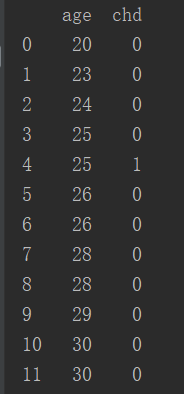
file = open("冠心病/CHD.csv")
data = pd.read_csv(file,header=0)
print(data) #输出数据集
print(data.describe()) #输出数据集的详细信息,均值,极值等
#绘制数据表示图
plt.figure() # Create a new figure
plt.axis([0,70,-0.2,1.2]) #坐标轴x从0~70,y从-0.2~1.2
plt.title('Original data')
plt.scatter(data['age'],data['chd'])
plt.show()
# 数据中心零均值处理
plt.figure()
plt.axis([-30,30,-0.2,1.2])
plt.title('Zero mean')
plt.scatter(data['age']-44.38 ,data['chd']) #44.38是数据均值
plt.show()
#数据标准差缩放处理
plt.figure()
plt.axis([-5,5,-0.2,1.2])
plt.title('Scaled by std dev')
plt.scatter((data['age']-44.38)/11.7,data['chd']) #11.7是数据方差
plt.show()
print('\n',(data['age']/11.721327).describe())输出结果:图1是数据显示。图2是数据详细信息。图3是原始数据图像显示。图4是数据中心零均值处理。图5是数据标准差缩放处理。


learning_rate = 0.2
training_epochs = 5   # 将训练数据分为 5个训练迭代循环,即5个epochs,
batch_size = 100
display_step = 1 # 每几个 epoch 画一次图
sess = tf.Session()
b = np.zeros((100,2))    # 100 行 2 列,全 0
#one-hot编码,这里只是先用来说明一下tf.one_hat的使用方法
print('列表 [1,3,2,4] 的 one-hot 编码为: \n\n',sess.run(tf.one_hot(indices=[1,3,2,4],depth=5,on_value= 1,off_value=0,axis=1,name='a')))

x = tf.placeholder('float',[None,1])    # 数据的第一列, Placeholder for the 1D data, 前面的 None 可以根据后面 Feed 自适应
y = tf.placeholder('float',[None,2])    # 数据的第二列
W = tf.Variable(tf.zeros([1,2]))    # [[0],[0]]
b = tf.Variable(tf.zeros([2]))      #   [0,0]
# 我们创建激活函数,并且将其作用于线性方程之上
activation = tf.nn.softmax(tf.matmul(x,W) + b)
# Minimize erroe using cross entropy
# 我们选择交叉熵作为损失函数,定义有优化器操作,选择梯度下降算法。
cost = tf.reduce_mean(-tf.reduce_sum(y*tf.log(activation),reduction_indices=1)) # Cross entropy
optimizer = tf.train.GradientDescentOptimizer(learning_rate).minimize(cost)  # Gradient Descent
init = tf.global_variables_initializer()

with tf.Session() as sess:
    tf.train.write_graph(sess.graph,'./Logist_one/','graph.pbtxt')
    sess.run(init)
    writer = tf.summary.FileWriter('./Logist_one/',sess.graph)
    # Initialize the drawing graph structure初始化绘图图结构
    graphnumber = 1
    plt.figure()# Generate a new graph
    # Iterate through all the epochs遍历
    for epoch in range(training_epochs):
        avg_cost = 0.
        total_batch = 400 // batch_size  # Loop over all batches
        for i in range(total_batch):
            # Transform the array into a one hot format
            # 由 API 可知 因为 axis = -1,故shape 为 features x depth,此外 deep 一般选择 indices 加一
            temp = tf.one_hot(indices=data['chd'].values, depth=2, on_value = 1, off_value = 0, axis = -1 , name = "a")
            # 由此说明 前面站位符处定义的 shape 和 Feed 的 shape 要保持一样才行
            # batch_xs, batch_ys = (data['age'].T - 44.38) / 11.721327, temp
            batch_xs, batch_ys = (np.transpose([data['age']])- 44.38)/11.721327, temp
            # Fit training using batch data
            sess.run(optimizer,feed_dict={x: batch_xs.astype(float),y: batch_ys.eval()})
            # Compute average loss, suming the corrent cost divided by the batch total number
            avg_cost += sess.run(cost,feed_dict={x: batch_xs.astype(float),y: batch_ys.eval()})/total_batch
        # Display logs per epoch step
        if epoch % display_step == 0:
            print('Epoch:', '%05d'%(epoch + 1), 'cost=',"{:.8f}".format(avg_cost))
            # Generate a new graph, and add it to the complete graph
            trX = np.linspace(-30, 30, 100)  #在指定的间隔内返回均匀间隔的数字
            print(b.eval())
            print(W.eval())
            Wdos = 2*W.eval()[0][0]/11.721327
            bdos = 2*b.eval()[0]
        # Cenerate the probability function (即广义化了的 Sigmoid 函数)
            trY = np.exp(-(Wdos*trX)+bdos)/(1+np.exp(-(Wdos*trX)+bdos))
        # Draw the samples and the probability function, whithout the normalization
            plt.subplots(graphnumber)
            #graphnumber = graphnumber + 1
            #Plot a scatter draw of the random datapoints
            plt.scatter(data['age'],data['chd'])
            plt.plot(trX+44.38,trY)    #  Plot a scatter draw of the random datapoints
            plt.title("logistic regression")
            plt.grid(True)
            plt.show()
        # Plot the final graph
        plt.savefig('test.svg')
输出结果:


