卷积神经网络层次结构包括:
数据输入层/ Input layer
卷积计算层/ CONV layer
激励层 / ReLU layer
池化层 / Pooling layer
全连接层 / FC layer
输入层(Input layer)
输入数据,通常会作一些数据处理,例如:
归一化:幅度归一化到同一范围
卷积计算层(CONV layer)
如上图图所示,左边为数据集,右边为一个神经网络
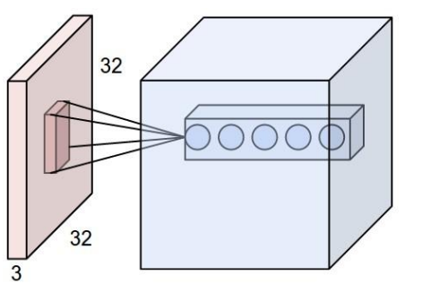
窗口:卷积计算层会在数据集上选定一个窗口,从窗口内选择数据
深度(depth):如下图所示,左边的数据集深度为3,右边的神经网络深度为5(有五个神经元)
步长(stride):窗口每次移动的距离
填充值(zero-padding):因为窗口移动到数据边缘时,可能不能正好遍历完所有数据,所以有时要在数据集周边填充上若干圈全为0的数据
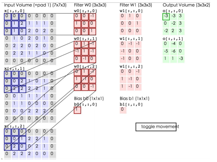
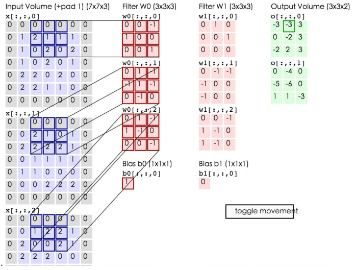
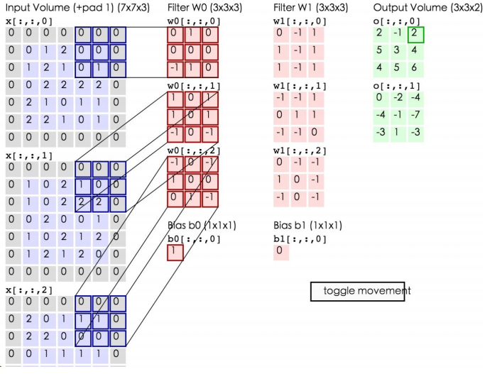
如上所示,左边为输入数据,中间为两个神经元,右边为输出。可以看到左边的输入数据中,窗口大小为3*3,每次移动的步长为2,周围有一层的填充数据,深度为3。中间为两个Filter,也就是线性方程的系数,注意Filter下面还有两个Bias偏移量。将窗口中的数据分别和Filter中的数据做卷积运算(即对应位置的数据相乘),再加上Bias偏移量即可得到一个输出矩阵中的一个值。比如在第一幅图的第三个窗口中的数据与Filter W0所做的运算为:
第一个窗口:0*0+0*0+0*(-1)+0*1+1*0+2*0+0*1+1*0+0*1=0
第二个窗口:0*0+0*1+0*(-1)+0*(-1)+0*1+2*(-1)+0*0+2*(-1)+2*0=-4
第三个窗口:0*0+0*1+0*(-1)+0*1+0*(-1)+1*0+0*0+2*0+0*(-1)=0
将这三个窗口中的值加起来再加上偏移量即得到了输出值:0+(-4)+0+1(偏移量)=-3,即第一个输出矩阵中的第一个值。
通过卷积层的计算后,可以使数据量大大减少,并且能够一定程度上保存数据集的信息
激励层
激励层的主要作用是将卷积层的结果做非线性映射。常见的激励层函数有sigmoid、tanh、Relu、Leaky Relu、ELU、Maxout
sigmoid函数如下所示:
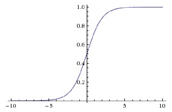
ReLu函数的有点是收敛非常快,因为在原点右侧它的偏导数为1,求导简单,这样在做反向传播时速度比较快。缺点时较为脆弱,原点左侧的函数具有的sigmoid相似的问题,即导数等于0。
Leaky ReLu在是ReLu的“增强版”,其函数表达式为:f(x)=max(ax,x),a通常为一个比较小的数,比如0.01,线面是a=0.01时的图像:
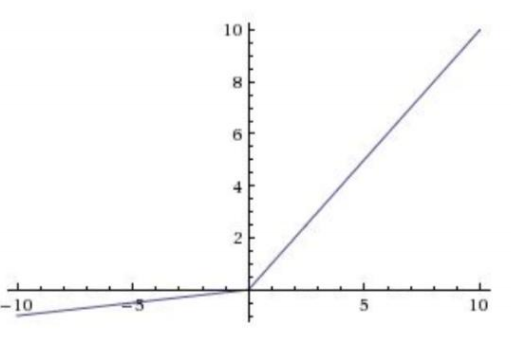
可以看到,相比ReLu,Leaky ReLu在原点左侧的表达式中对x乘以了一个比较小的系数,这样保证了在做反向传播时不会挂掉,并且其计算也很快。
激励函数使用总结:
1.尽量不要用sigmoid函数
2.首选ReLu,速度快,但是需要小心,有可能会挂掉
3.ReLu不行的话再选用Leaky ReLu或者Maxout
池化层(Pooling layer)
在连续的卷基层和激励层中间,用于压缩数据和参数的量,用于减少过拟合。
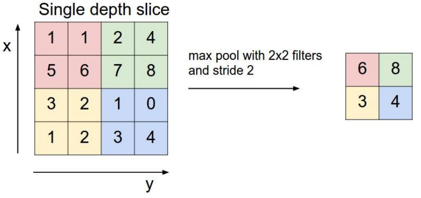
池化层的选择策略有max pooling和average Pooling,上图展示的就是max Pooling的过程。在原始的数据层上划分一个个小块,在每个小块中选择最大的那个数代表这个小块中所有的数(如果是average Pooling就选择平均数),放到下一层。这样就打打减少了数据量。这种做法的理论依据好像还不太清楚,但是可以想象在一幅图中,每个像素点和其周边的点大致是一样的,所以用一个点代替其周边点也有一定道理。
全连接层(FC layer)
全连接层即两层之间的所有神经元都有权重连接,通常会在卷积神经网络的尾部。
---------------------
作者:一路前行1
来源:CSDN
原文:https://blog.csdn.net/weiyongle1996/article/details/78088654
版权声明:本文为博主原创文章,转载请附上博文链接!
import torch
import torch.nn as nn
import torch.nn.functional as F
"""
Neural networks can be constructed using the torch.nn package.
nn depends on autograd to define models and differentiate them.
An nn.Module contains layers, and a method forward(input)that returns the output.
"""


class Net(nn.Module):
    def __init__(self):
        super(Net, self).__init__()
        # 1 input image channel, 6 output channels, 5x5 square convolution
        self.conv1 = nn.Conv2d(in_channels=1, out_channels=6, kernel_size=5)
        print(self.conv1.weight.data)
        self.conv2 = nn.Conv2d(in_channels=6, out_channels=16, kernel_size=5)
        print(self.conv2.weight.data)
        # an affine仿射 operation: y = Wx + b ;
        # class torch.nn.Linear(in_features, out_features, bias=True)
        # in_features - 每个输入样本的大小 out_features - 每个输出样本的大小
        self.fc1 = nn.Linear(16*5*5, 120)                          # 为啥是16*5*5
        print(self.fc1.weight.data, self.fc1.weight.size())
        self.fc2 = nn.Linear(120, 84)
        self.fc3 = nn.Linear(84, 10)

    def forward(self, x):
        # Max pooling over a (2, 2) window
        x = F.max_pool2d(F.relu(self.conv1(x)), (2, 2))
        # If the size is a square you can only specify a single number
        x = F.max_pool2d(F.relu(self.conv2(x)), (2, 2))
        print(x)
        x = x.view(-1, self.num_flat_features(x))  # 代表what
        x = F.relu(self.fc1(x))
        x = F.relu(self.fc2(x))
        x = self.fc3(x)
        return x

    def num_flat_features(self, x):           # 特征展开
        print(x.size(), "************")
        size = x.size()[1:]
        print("--------%s", size)
        num_features = 1
        for s in size:
            num_features *= s
        return num_features


net = Net()
print(net)

"""
You just have to define the forward function,
and the backward function (where gradients are computed) is automatically defined for you using autograd.
You can use any of the Tensor operations in the forward function.
"""
# The learnable parameters of a model are returned by net.parameters()
"""
如何计算CNN的每层参数个数
"""
params = list(net.parameters())
print(list(params))
print(len(params))
print(params[0].size(), params[1].size(), params[2].size())  # conv1's .weight ...

input = torch.randn(1, 1, 32, 32)
print(input)
out = net(input)
print(out)

net.zero_grad()
out.backward(torch.randn(1, 10))
"""
torch.nn only supports mini-batches.
The entire torch.nn package only supports inputs that are a mini-batch of samples, and not a single sample.
For example, nn.Conv2d will take in a 4D Tensor of nSamples x nChannels x Height x Width.
"""

output = net(input)
target = torch.randn(10)  # a dummy target, for example
target = target.view(1, -1)   # 在不改变张量数据的情况下随意改变张量的大小和形状
criterion = nn.MSELoss()

loss = criterion(output, target)
print(loss)

print(loss.grad_fn)              # MSELoss
print(loss.grad_fn.next_functions[0][0])         # Linear
print(loss.grad_fn.next_functions[0][0].next_functions[0][0])  # ReLU

"""
To backpropagate the error all we have to do is to loss.backward().
You need to clear the existing gradients though, else gradients will be accumulated to existing gradients.
"""

# net.zero_grad()
# print('conv1.bias.grad before backward')
# # print(net.conv1.weight.grad)
# print(net.conv1.bias.grad)
# loss.backward()
# print('conv1.bias.grad after backward')
# # print(net.conv1.weight.grad)
# print(net.conv1.bias.grad)

"""
The simplest update rule used in practice is the Stochastic Gradient Descent (SGD):
weight = weight - learning_rate * gradient
UPDATE THE WEIGHTS
"""
learning_rate = 0.01
for f in net.parameters():
    f.data.sub_(f.grad.data * learning_rate)
"""
To enable to use various different update rules such as SGD, Nesterov-SGD, Adam, RMSProp, etc.
builting a small package: torch.optim that implements all these methods. Using it is very simple:
"""

import torch.optim as optim

# create your optimizer
optimizer = optim.SGD(net.parameters(), learning_rate)

# in your training loop
optimizer.zero_grad()
output = net(input)
loss = criterion(output, target)    # zero the gradient buffers
loss.backward()
optimizer.step()       # Does the update


"""
Define the network
loss function
Backprop
Update the weights
"""