机器学习之类别不平衡问题 —— ROC和PR曲线

写在前面：在CTR预估中，用户发生点击行为这类正样本显著少于负样本，那么用ROC来评价通常结果非常乐观，在网上调研了两天，对于不平衡问题，有多重评价方法，尤其是PR曲线最常用，无论是竞赛还是实际场景中，这篇文章总结的非常全面，转载到这。

机器学习之类别不平衡问题 (2) —— ROC和PR曲线

完整代码

ROC曲线和PR（Precision - Recall）曲线皆为类别不平衡问题中常用的评估方法，二者既有相同也有不同点。本篇文章先给出ROC曲线的概述、实现方法、优缺点，再阐述PR曲线的各项特点，最后给出两种方法各自的使用场景。

ROC曲线

ROC曲线常用于二分类问题中的模型比较，主要表现为一种真正例率 (TPR) 和假正例率 (FPR) 的权衡。具体方法是在不同的分类阈值 (threshold) 设定下分别以TPR和FPR为纵、横轴作图。由ROC曲线的两个指标，TPR=TPP=TPTP+FN。最后的到所有样本点的TPR和FPR值，用线段相连。

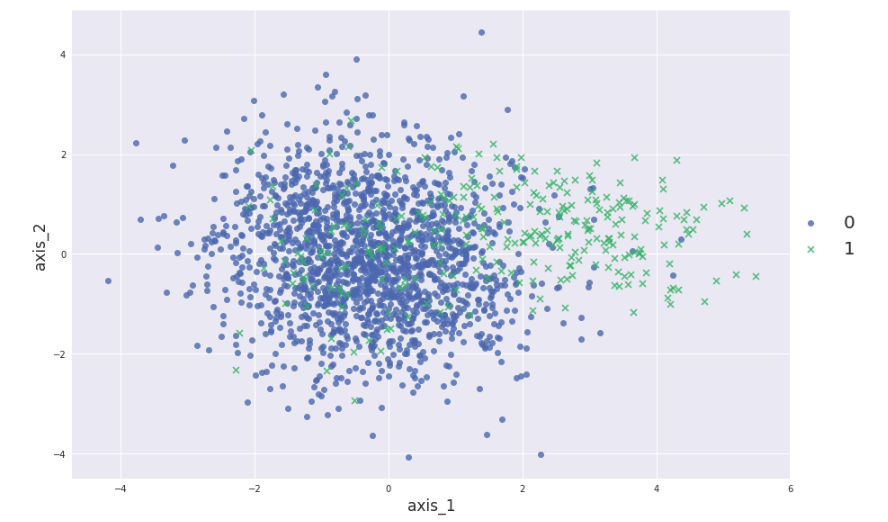
下面进行实现，先模拟生成一个正例：负例=10：1的数据集，用PCA降到2维进行可视化：

X,y = make_classification(n_samples=2000, n_features=10, n_informative=4,
                         n_redundant=1, n_classes=2, n_clusters_per_class=1,
                         weights=[0.9,0.1], flip_y=0.1, random_state=2018)

sns.lmplot(“pca_a”,“pca_b”,data=X_pca, hue=“y”, fit_reg=False, markers=[“o”,“x”],size=8,aspect=1.5,legend=False)
plt.legend(fontsize=20,bbox_to_anchor=(0.98, 0.6),edgecolor =‘r’)
plt.xlabel(“axis_1”,fontsize=17)
plt.ylabel(“axis_2”,fontsize=17)

将数据分成训练集和测试集，使用Logistic Regression和Random Forest作图：

kf = StratifiedKFold(n_splits=2, random_state=42)
for train_index, test_index in kf.split(X,y):
    X_train, X_test = X[train_index], X[test_index]
    y_train, y_test = y[train_index], y[test_index]

lr = LogisticRegression()
lr.fit(X_train,y_train)
pos_prob_lr = lr.predict_proba(X_test)[:,1] # Logistic Regression的正例预测概率

rf = RandomForestClassifier(random_state=42)
rf.fit(X_train,y_train)
pos_prob_rf = rf.predict_proba(X_test)[:,1] # Random Forest的正例预测概率

def get_roc(pos_prob,y_true):
pos = y_true[y_true==1]
neg = y_true[y_true==0]
threshold = np.sort(pos_prob)[::-1] # 按概率大小逆序排列
y = y_true[pos_prob.argsort()[::-1]]
tpr_all = [0] ; fpr_all = [0]
tpr = 0 ; fpr = 0
x_step = 1/float(len(neg))
y_step = 1/float(len(pos))
y_sum = 0 # 用于计算AUC
for i in range(len(threshold)):
if y[i] == 1:
tpr += y_step
tpr_all.append(tpr)
fpr_all.append(fpr)
else:
fpr += x_step
fpr_all.append(fpr)
tpr_all.append(tpr)
y_sum += tpr
return tpr_all,fpr_all,y_sum*x_step # 获得总体TPR，FPR和相应的AUC

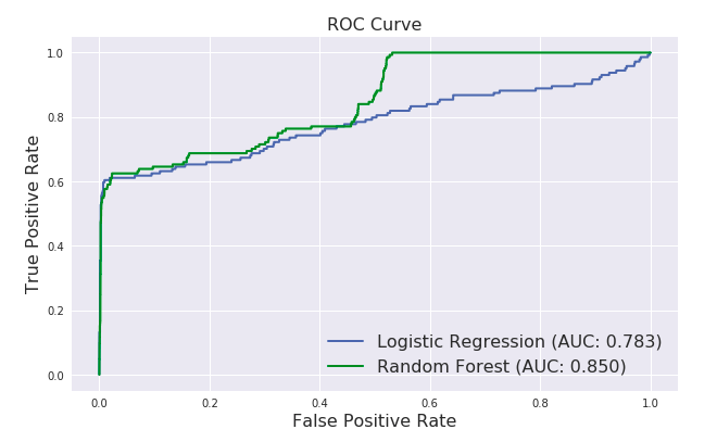
tpr_lr,fpr_lr,auc_lr = get_roc(pos_prob_lr,y_test)
tpr_rf,fpr_rf,auc_rf = get_roc(pos_prob_rf,y_test)

plt.figure(figsize=(10,6))
plt.plot(fpr_lr,tpr_lr,label=“Logistic Regression (AUC: {:.3f})”.format(auc_lr),linewidth=2)
plt.plot(fpr_rf,tpr_rf,‘g’,label=“Random Forest (AUC: {:.3f})”.format(auc_rf),linewidth=2)
plt.xlabel(“False Positive Rate”,fontsize=16)
plt.ylabel(“True Positive Rate”,fontsize=16)
plt.title(“ROC Curve”,fontsize=16)
plt.legend(loc=“lower right”,fontsize=16)

ROC曲线的优点

放一张混淆矩阵图可能看得更清楚一点 :

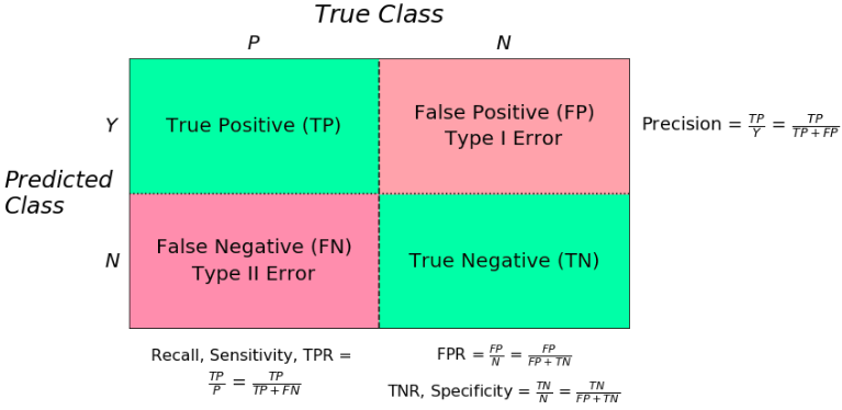
兼顾正例和负例的权衡。因为TPR聚焦于正例，FPR聚焦于与负例，使其成为一个比较均衡的评估方法。
ROC曲线选用的两个指标，TPR=TPP=TPTP+FN，都不依赖于具体的类别分布。

注意TPR用到的TP和FN同属P列，FPR用到的FP和TN同属N列，所以即使P或N的整体数量发生了改变，也不会影响到另一列。也就是说，即使正例与负例的比例发生了很大变化，ROC曲线也不会产生大的变化，而像Precision使用的TP和FP就分属两列，则易受类别分布改变的影响。

参考文献 [1] 中举了个例子，负例增加了10倍，ROC曲线没有改变，而PR曲线则变了很多。作者认为这是ROC曲线的优点，即具有鲁棒性，在类别分布发生明显改变的情况下依然能客观地识别出较好的分类器。

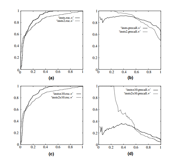
下面我们来验证一下是不是这样：

X_test_dup = np.vstack((X_test,X_test[y_test==0],X_test[y_test==0],X_test[y_test==0],X_test[y_test==0],X_test[y_test==0],X_test[y_test==0],X_test[y_test==0],X_test[y_test==0],X_test[y_test==0]))
y_test_dup = np.array(y_test.tolist() + y_test[y_test==0].tolist()*9)   # 10x倍负例的测试集

pos_prob_lr_dup = lr.predict_proba(X_test_dup)[:,1]
pos_prob_rf_dup = rf.predict_proba(X_test_dup)[:,1]
tpr_lr_dup,fpr_lr_dup,auc_lr_dup = get_roc(pos_prob_lr_dup,y_test_dup)
tpr_rf_dup,fpr_rf_dup,auc_rf_dup = get_roc(pos_prob_rf_dup,y_test_dup)

plt.figure(figsize=(10,6))
plt.plot(fpr_lr_dup,tpr_lr_dup,label=“Logistic Regression (AUC: {:.3f})”.format(auc_lr_dup),linewidth=2)
plt.plot(fpr_rf_dup,tpr_rf_dup,‘g’,label=“Random Forest (AUC: {:.3f})”.format(auc_rf_dup),linewidth=2)
plt.xlabel(“False Positive Rate”,fontsize=16)
plt.ylabel(“True Positive Rate”,fontsize=16)
plt.title(“ROC Curve”,fontsize=16)
plt.legend(loc=“lower right”,fontsize=16)

Logistic Regression的曲线几乎和先前一模一样，但Random Forest的曲线却产生了很大变化。个中原因看一下两个分类器的预测概率就明白了：

pos_prob_lr_dup[:20]
array([0.15813023, 0.12075471, 0.02763748, 0.00983065, 0.06201179,
       0.04986294, 0.09926128, 0.05632981, 0.15558692, 0.05856262,
       0.08661055, 0.00787402, 0.1617371 , 0.04063957, 0.14103442,
       0.07734239, 0.0213237 , 0.03968638, 0.03771455, 0.04874451])

pos_prob_rf_dup[:20]
array([0. , 0. , 0.1, 0.1, 0. , 0.1, 0.2, 0. , 0.1, 0.1, 0.1, 0. , 0. ,
       0.2, 0. , 0. , 0.2, 0. , 0.1, 0. ])

可以看到Logistic Regression的预测概率几乎没有重复，而Random Forest的预测概率则有很多重复，因为Logistic Regression可以天然输出概率，而Random Forest本质上属于树模型，只能输出离散值。scikit-learn中树模型的predict_proba() 方法表示的是一个叶节点上某一类别的样本比例，但只显示小数点后一位，致使大量样本的预测概率都一样。当画ROC曲线时需要先将样本根据预测概率排序，若几个样本的概率一样，则只能按原来的顺序排列。上面的操作就是将所有累加的负例都排在了原始数据后面，致使正例的顺序都很靠前，造成Random Forest的结果好了不少。解决办法就是将所有样本随机排序，就能产生和原来差不多的ROC曲线了：

index = np.random.permutation(len(X_test_dup))
X_test_dup = X_test_dup[index]
y_test_dup = y_test_dup[index]

ROC曲线的缺点

上文提到ROC曲线的优点是不会随着类别分布的改变而改变，但这在某种程度上也是其缺点。因为负例N增加了很多，而曲线却没变，这等于产生了大量FP。像信息检索中如果主要关心正例的预测准确性的话，这就不可接受了。

在类别不平衡的背景下，负例的数目众多致使FPR的增长不明显，导致ROC曲线呈现一个过分乐观的效果估计。ROC曲线的横轴采用FPR，根据FPR = FPN

下面仍使用上面的数据集画图：

def get_pr(pos_prob,y_true):
    pos = y_true[y_true==1]
    threshold = np.sort(pos_prob)[::-1]
    y = y_true[pos_prob.argsort()[::-1]]
    recall = [] ; precision = []
    tp = 0 ; fp = 0
    auc = 0
    for i in range(len(threshold)):
        if y[i] == 1:
            tp += 1
            recall.append(tp/len(pos))
            precision.append(tp/(tp+fp))
            auc += (recall[i]-recall[i-1])*precision[i]
        else:
            fp += 1
            recall.append(tp/len(pos))
            precision.append(tp/(tp+fp))
    return precision,recall,auc

precision_lr,recall_lr,auc_lr = get_pr(pos_prob_lr,y_test)
precision_rf,recall_rf,auc_rf = get_pr(pos_prob_rf,y_test)

plt.figure(figsize=(10,6))
plt.plot(recall_lr,precision_lr,label=“Logistic Regression (AUC: {:.3f})”.format(auc_lr),linewidth=2)
plt.plot(recall_rf,precision_rf,label=“Random Forest (AUC: {:.3f})”.format(auc_rf),linewidth=2)
plt.xlabel(“Recall”,fontsize=16)
plt.ylabel(“Precision”,fontsize=16)
plt.title(“Precision Recall Curve”,fontsize=17)
plt.legend(fontsize=16)

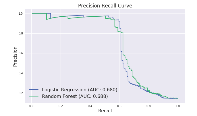
可以看到上文中ROC曲线下的AUC面积在0.8左右，而PR曲线下的AUC面积在0.68左右，类别不平衡问题中ROC曲线确实会作出一个比较乐观的估计，而PR曲线则因为Precision的存在会不断显现FP的影响。

使用场景

ROC曲线由于兼顾正例与负例，所以适用于评估分类器的整体性能，相比而言PR曲线完全聚焦于正例。
如果有多份数据且存在不同的类别分布，比如信用卡欺诈问题中每个月正例和负例的比例可能都不相同，这时候如果只想单纯地比较分类器的性能且剔除类别分布改变的影响，则ROC曲线比较适合，因为类别分布改变可能使得PR曲线发生变化时好时坏，这种时候难以进行模型比较；反之，如果想测试不同类别分布下对分类器的性能的影响，则PR曲线比较适合。
如果想要评估在相同的类别分布下正例的预测情况，则宜选PR曲线。
类别不平衡问题中，ROC曲线通常会给出一个乐观的效果估计，所以大部分时候还是PR曲线更好。
最后可以根据具体的应用，在曲线上找到最优的点，得到相对应的precision，recall，f1 score等指标，去调整模型的阈值，从而得到一个符合具体应用的模型。

Reference:

Tom Fawcett. An introduction to ROC analysis
Jesse Davis, Mark Goadrich0 The Relationship Between Precision-Recall and ROC Curves
Haibo He, Edwardo A. Garcia. Learning from Imbalanced Data
周志华. 《机器学习》
Pang-Ning Tan, etc. Introduction to Data Mining
https://stats.stackexchange.com/questions/7207/roc-vs-precision-and-recall-curves

转载自https://www.cnblogs.com/massquantity/p/8592091.html