机器学习中的ROC和PR曲线以及代码实现

转自：https://blog.csdn.net/taoyanqi8932/article/details/54409314

引言

 在 21 Must-Know Data Science Interview Questions and Answers 的文章中，有这类似这样的问题，它问的是Explain what precision and recall are. How do they relate to the ROC curve?关于这个问题其实有许多需要回答的，不仅仅是他们的表现形式不同，同时它涉及到下机器学习中的性能度量(performance measure)问题，下面对其进行详细的说明。

性能度量(performance measure)

在对学习器的泛化能力进行评估是模型泛化的能力，即要用到机器学习的性能度量，不同的性能度量往往会导致不同的评判结果，这意味着模型的好坏事相对的，什么样的模型是好的，不仅取决于算法和数据，还决定于任务的需求。 
最常见的的分类中所用的度量是：accuracy(准确度)，error rate

acc=1m∑i=1mI(f(xi)=yi)acc=1m∑i=1mI(f(xi)=yi)

err=1m∑i=1mI(f(xi)≠yi)err=1m∑i=1mI(f(xi)≠yi)

上面两种度量方法非常的常用，但是有时并不能满足任务的要求，其准确度将每个类看得同等的重要，因此它可能不适合用来分析不平衡的数据集，不平衡的数据集即正类样本远远小于负类的样本，但是我们用对正类的样本比较关心，这样准确度就不适合这种度量了，因此引入了下面的几种度量方法。

假定下面一个例子，假定在10000个样本中有100个正样本，其余为负样本，其在分类器下的混淆矩阵(confusion matrix)为：

则，我们定义：

1. TN / True Negative: case was negative and predicted negative 
2. TP / True Positive: case was positive and predicted positive 
3. FN / False Negative: case was positive but predicted negative 
4. FP / False Positive: case was negative but predicted positive

扫描二维码关注公众号，回复： 2065858 查看本文章

则定义一下度量：

真正率(true positive rate,TPR)或灵敏度(sensitivity)，定义为被模型正确预测的正样本的比例：

TPR=TPTP+FNTPR=TPTP+FN

真负率(true negative rate,TFR)或特指度(specificity)，定义为被模型正确预测的负样本的比例： 

TPR=TNTN+FPTPR=TNTN+FP

同理，假正率(false positive rate,FPR) 

FPR=FPTN+FPFPR=FPTN+FP

假负率(flase negative rate,FNR) 

FNR=FNTP+FNFNR=FNTP+FN

重要的两个度量：

precision(精度)，其与accuracy感觉中文翻译一致，周志华老师的书中称为：查准率:

p=TPTP+FPp=TPTP+FP

recall(召回率),周志华老师的书中称为查全率，其又与真正率一个公式： 

r=TPTP+FNr=TPTP+FN

精度是确定分类器中断言为正样本的部分其实际中属于正样本的比例，精度越高则假的正例就越低，召回率则是被分类器正确预测的正样本的比例。两者是一对矛盾的度量，其可以合并成令一个度量，F1度量： 

F1=2rpr+p=2∗TP2∗TP+FP+FNF1=2rpr+p=2∗TP2∗TP+FP+FN

如果对于precision和recall的重视不同，则一般的形式： 

Fβ=(1+β2)rpβ2∗p+rFβ=(1+β2)rpβ2∗p+r

可以从公式中看到 β=1β=1 则退化成F1, β>1β>1 则recall有更大影响，反之则precision更多影响。

维基百科中一个非常好的关于两者之间的例子：

有了上面的知识，就可以理解ROC,和PRC了。

ROC and PRC

ROC(receiver operating characteristic)接受者操作特征，其显示的是分类器的真正率和假正率之间的关系，如下图所示：

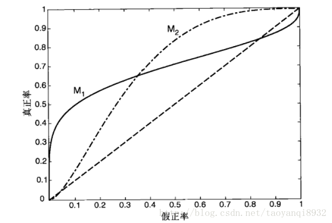
ROC曲线有助于比较不同分类器的相对性能，当FPR小于0.36时M1浩宇M2，而大于0.36是M2较好。 
ROC曲线小猫的面积为AUC(area under curve)，其面积越大则分类的性能越好，理想的分类器auc=1。

PR(precision recall)曲线表现的是precision和recall之间的关系，如图所示：

如何选择ROC,PR

下面节选自：What is the difference between a ROC curve and a precision-recall curve? When should I use each?

Particularly, if true negative is not much valuable to the problem, or negative examples are abundant. Then, PR-curve is typically more appropriate. For example, if the class is highly imbalanced and positive samples are very rare, then use PR-curve. One example may be fraud detection, where non-fraud sample may be 10000 and fraud sample may be below 100. 
In other cases, ROC curve will be more helpful.

其说明，如果是不平衡类，正样本的数目非常的稀有，而且很重要，比如说在诈骗交易的检测中，大部分的交易都是正常的，但是少量的非正常交易确很重要。

Let’s take an example of fraud detection problem where there are 100 frauds out of 2 million samples. 
Algorithm 1: 90 relevant out of 100 identified 
Algorithm 2: 90 relevant out of 1000 identified

Evidently, algorithm 1 is more preferable because it identified less number of false positive. 
In the context of ROC curve, 
Algorithm 1: TPR=90/100=0.9, FPR= 10/1,999,900=0.00000500025 
Algorithm 2: TPR=90/100=0.9, FPR=910/1,999,900=0.00045502275 
The FPR difference is 0.0004500225

For PR, Curve 
Algorithm 1: precision=0.9, recall=0.9 
Algorithm 2: Precision=90/1000=0.09, recall= 0.9 
Precision difference= 0.81

可以看到在正样本非常少的情况下，PR表现的效果会更好。

如何绘制ROC曲线

为了绘制ROC曲线，则分类器应该能输出连续的值，比如在逻辑回归分类器中，其以概率的形式输出，可以设定阈值大于0.5为正样本，否则为负样本。因此设置不同的阈值就可以得到不同的ROC曲线中的点。 
下面给出具体的实现过程：

来源：数据挖掘导论

下面给出sklearn中的实现过程：

print(__doc__)

import numpy as np
from scipy import interp
import matplotlib.pyplot as plt
from itertools import cycle

from sklearn import svm, datasets
from sklearn.metrics import roc_curve, auc
from sklearn.model_selection import StratifiedKFold

###############################################################################
# Data IO and generation

# import some data to play with
iris = datasets.load_iris()
X = iris.data
y = iris.target
X, y = X[y != 2], y[y != 2]
n_samples, n_features = X.shape

# Add noisy features
random_state = np.random.RandomState(0)
X = np.c_[X, random_state.randn(n_samples, 200 * n_features)]

###############################################################################
# Classification and ROC analysis

# Run classifier with cross-validation and plot ROC curves
cv = StratifiedKFold(n_splits=6)

# 注意这里的应该改为probability=True以概率形式输出
classifier = svm.SVC(kernel='linear', probability=True,
                     random_state=random_state)

mean_tpr = 0.0
mean_fpr = np.linspace(0, 1, 100)

colors = cycle(['cyan', 'indigo', 'seagreen', 'yellow', 'blue', 'darkorange'])
lw = 2

i = 0
# k折交叉验证
for (train, test), color in zip(cv.split(X, y), colors):
    probas_ = classifier.fit(X[train], y[train]).predict_proba(X[test])
    # Compute ROC curve and area the curve
    #　注意这里返回的阈值，以区分正负样本的阈值
    fpr, tpr, thresholds = roc_curve(y[test], probas_[:, 1])
    ＃　进行插值
    mean_tpr += interp(mean_fpr, fpr, tpr)
    mean_tpr[0] = 0.0
    roc_auc = auc(fpr, tpr)
    plt.plot(fpr, tpr, lw=lw, color=color,
             label='ROC fold %d (area = %0.2f)' % (i, roc_auc))

    i += 1
plt.plot([0, 1], [0, 1], linestyle='--', lw=lw, color='k',
         label='Luck')

mean_tpr /= cv.get_n_splits(X, y)
mean_tpr[-1] = 1.0
mean_auc = auc(mean_fpr, mean_tpr)
plt.plot(mean_fpr, mean_tpr, color='g', linestyle='--',
         label='Mean ROC (area = %0.2f)' % mean_auc, lw=lw)

plt.xlim([-0.05, 1.05])
plt.ylim([-0.05, 1.05])
plt.xlabel('False Positive Rate')
plt.ylabel('True Positive Rate')
plt.title('Receiver operating characteristic example')
plt.legend(loc="lower right")
plt.show()

• 1
• 2
• 3
• 4
• 5
• 6
• 7
• 8
• 9
• 10
• 11
• 12
• 13
• 14
• 15
• 16
• 17
• 18
• 19
• 20
• 21
• 22
• 23
• 24
• 25
• 26
• 27
• 28
• 29
• 30
• 31
• 32
• 33
• 34
• 35
• 36
• 37
• 38
• 39
• 40
• 41
• 42
• 43
• 44
• 45
• 46
• 47
• 48
• 49
• 50
• 51
• 52
• 53
• 54
• 55
• 56
• 57
• 58
• 59
• 60
• 61
• 62
• 63
• 64
• 65
• 66
• 67
• 68
• 69
• 70
• 71
• 72

运行的结果如下图所示：

参考资料：

１.《机器学习》周志华 
２.《数据挖掘导论》 
３. 21 Must-Know Data Science Interview Questions and Answers 
４. What is the difference between a ROC curve and a precision-recall curve? When should I use each? 
5. Receiver Operating Characteristic (ROC) with cross validation