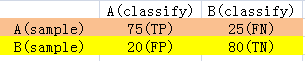
对于二分类问题,它的样本只有正样本和负样本两类。测试样本中,正样本被分类器判定为正样本的数量记为TP(true positive),被判定为负样本的数量记为FP(false negative)。负样本被分类器判定为负样本的数量记为TN(true negative),被判定为正样本的数量记为FP(false positive)。如图所示,A,B两组样本总数量各为100。
精度定义: TP/(TP+FP)
召回率定义:TP/(TP+FN)
虚景率: 1 - TP/(TP+FP)
真阳率:TPR =TP/(TP +FN)
假阳率:FPR = FP/(FP+TN)
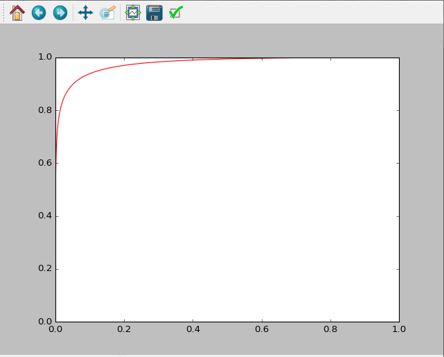
ROS曲线的横轴为假阳率,纵轴为真阳率。
一个好的分类曲线应该让假阳率低,真阳率高,理想情况下应该是接近于y=1 的直线,即让曲线下的面积尽可能的大。
例子:
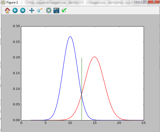
生成两组正态分布样本,两组样本对应的标签分别表示正样本,和负样本;资源链接如下:
链接:https://pan.baidu.com/s/1X4hHygzSQHB3f8_kepxE8A
提取码:6uvg
# -*- coding: utf-8 -*-
"""
Spyder Editor

This is a temporary script file.
"""
import numpy as np
import matplotlib.pyplot as plt
from scipy import stats

def floatrange(start,stop,steps):
    return [start+float(i)*(stop-start)/(float(steps)-1) for i in range(steps)]

"""读取数据"""
data = np.loadtxt('data.txt')

""""计算不同类别的正态参数"""
totalCount = len(data[:,0])
positiveCount =np.sum(data[:,1])
negativeCount = totalCount - positiveCount

#正标本均值,方差
positiveIndex= np.where(data[:,1] ==1)
positiveSum = np.sum(data[positiveIndex,0])
positive_u =positiveSum / positiveCount
positive_derta =np.sqrt(np.sum(np.square(data[positiveIndex,0] - positive_u )) / positiveCount)

#负标本均值,方差
negativeIndex= np.where(data[:,1] ==0)
negativeSum = np.sum(data[negativeIndex,0])
negative_u =negativeSum / negativeCount
negative_derta =np.sqrt(np.sum(np.square(data[negativeIndex,0] - negative_u )) / negativeCount)

#概率密度 曲线绘制
x = floatrange(2,25,1000)
print(positive_u,positive_derta)
pd = np.exp(-1.0*np.square(x-positive_u) / (2*np.square(positive_derta))) /(positive_derta*np.sqrt(2*np.pi))
nd = np.exp(-1.0*np.square(x-negative_u) / (2*np.square(negative_derta))) /(negative_derta*np.sqrt(2*np.pi))
plt.figure(1)
plt.plot(x,pd,'r')
plt.plot(x,nd,'b')


#概率分布构建
positiveFun = stats.norm(positive_u,positive_derta)
negativeFun = stats.norm(negative_u,negative_derta)

positiveValue = positiveFun.cdf(x)
negativeValue = negativeFun.cdf(x)


#真阳率,假阳率
positiveRate = 1 -positiveFun.cdf(x)
negativeRate = 1 -negativeFun.cdf(x)

#阀值
disvalue =positiveFun.cdf(x) +1 -negativeFun.cdf(x)
minvalue = np.min(disvalue)
index = np.where(disvalue == minvalue)
indexvalue =int(index[0])

xvalue = x[indexvalue]

#混淆矩阵
positivevalue = 1 -positiveFun.cdf(xvalue)
negativevalue = 1 -negativeFun.cdf(xvalue)
v00= int(positivevalue * positiveCount)
v01= positiveCount -v00
v10 =int(negativevalue* negativeCount)
v11 =negativeCount -v10
print("disvalue:",xvalue)
print("positiverate:",positivevalue,"negativerate:",negativevalue)
print(v00,",",v01)
print(v10,",",v11)


xdis = [xvalue,xvalue]
ydis = [0,0.2]
plt.plot(xdis,ydis,'g')
"""ros 曲线"""
plt.figure(2)
plt.plot(negativeRate,positiveRate,'r')
运行结果如下所示: