以下笔记来源:Andrew Ng的卷积神经网络week1
在学习深度学习之前掌握其中的概念非常重要,列举一些在网络中经常遇到且容易混淆的名词。
1. 概念
Step: 训练模型的步数
Batch Size(批尺寸): 计算梯度所需的样本数量,太小会导致效率低下,无法收敛。太大会导致内存撑不住,Batch Size增大到一定程度后,其下降方向变化很小了,所以Batch Size是一个很重要的参数。
Epoch(回合):代表样本集内所有的数据经过了一次训练。
Iteration(迭代):理解迭代,只需要知道乘法表或者一个计算器就可以了。迭代是 batch 需要完成一个 epoch 的次数。记住:在一个 epoch 中,batch 数和迭代数是相等的。
eg.比如对于一个有 5000 个训练样本的数据集。将 5000 个样本分成大小为 500 的 batch,那么完成一个 epoch 需要 10 个 iteration。
参数/超参数:超参数包括学习率,hidden layer,激活函数,其余参数多数为参数
2.网络结构


卷积层:
- Zero Padding
- Convolve window
- Convolution forward
- Convolution backward (optional)
Zero-Padding
Zero-padding:在图像周围填0,如图

填充的主要好处如下:
它允许使用CONV层而不必缩小卷的高度和宽度。 这对于构建更深层的网络非常重要,否则高度/宽度会随着您进入更深层而缩小。 一个重要的特殊情况是“相同”卷积,其中高度/宽度在一层之后被精确保留。同时它也可以帮助我们将更多信息保存在图像的边界。 如果没有填充,则下一层中的极少数值会受到像素作为图像边缘的影响。
python实现填充函数
np.pad(X, ((0, 0),(pad, pad),(pad, pad),(0, 0)), 'constant', constant_values=0)Single step of convolution:

在这一部分中,实现一个卷积步骤,在此步骤中将滤波器应用于输入的单个位置。 这将用于构建卷积单元,其中:
获取输入体积
在输入的每个位置应用过滤器
输出另一个体积(通常是不同大小)
在计算机视觉应用中,左边的矩阵中的每个值对应于单个像素值,并且我们通过将其值与元素的原始矩阵相乘,然后将它们相加来将3x3滤波器与图像卷积。
# GRADED FUNCTION: conv_single_step

def conv_single_step(a_slice_prev, W, b):
    s = np.multiply(a_slice_prev, W) + b
    Z = np.sum(s)
    return Z
Forward pass

实现下面的函数在输入激活A_prev上卷积滤波器W. 该函数将输入A_prev,前一层的激活输出(对于一批m个输入),由W表示的F滤波器/权重,以及由b表示的偏置矢量,其中每个滤波器具有其自己的(单个)偏置。 最后,还可以访问包含步幅和填充的超参数字典。
# GRADED FUNCTION: conv_forward

def conv_forward(A_prev, W, b, hparameters):

    (m, n_H_prev, n_W_prev, n_C_prev) = A_prev.shape

    # Retrieve dimensions from W's shape (≈1 line)
    (f, f, n_C_prev, n_C) = W.shape

    # Retrieve information from "hparameters" (≈2 lines)
    stride = hparameters['stride']
    pad = hparameters['pad']

    # Compute the dimensions of the CONV output volume using the formula given above.
    n_H = 1 + int((n_H_prev + 2 * pad - f) / stride)
    n_W = 1 + int((n_W_prev + 2 * pad - f) / stride)

    # Initialize the output volume Z with zeros. (≈1 line)
    Z = np.zeros((m, n_H, n_W, n_C))

    # Create A_prev_pad by padding A_prev
    A_prev_pad = zero_pad(A_prev, pad)

    for i in range(m):
        a_prev_pad = A_prev_pad[i]
        for h in range(n_H):
            for w in range(n_W):
                for c in range(n_C):
                    vert_start = h * stride
                    vert_end = vert_start + f
                    horiz_start = w * stride
                    horiz_end = horiz_start + f

                    a_slice_prev = a_prev_pad[vert_start:vert_end, horiz_start:horiz_end, :]
                    Z[i, h, w, c] = np.sum(np.multiply(a_slice_prev, W[:, :, :, c]) + b[:, :, :, c])

    # Making sure your output shape is correct
    assert(Z.shape == (m, n_H, n_W, n_C))

    # Save information in "cache" for the backprop
    cache = (A_prev, W, b, hparameters)

    return Z, cache
池化层:
- Pooling forward
- Create mask
- Distribute value
- Pooling backward (optional)
作用:池化减小了输入的高度和宽度。 它有助于减少计算,并有助于使特征检测器在输入中的位置更加不变。
常用的两种类型的池层是:
最大池层:在输入上滑动窗口,并将窗口的最大值存储在输出中。
平均池层:在输入上滑动窗口,并在输出中存储窗口的平均值。

注:池化层没有参数需要训练,只有窗口的尺寸超差需要设置
Forward Pooling:
没有填充,将池的输出形状绑定到输入形状的公式为:

# GRADED FUNCTION: pool_forward

def pool_forward(A_prev, hparameters, mode = "max"):

    # Retrieve dimensions from the input shape
    (m, n_H_prev, n_W_prev, n_C_prev) = A_prev.shape

    # Retrieve hyperparameters from "hparameters"
    f = hparameters["f"]
    stride = hparameters["stride"]

    # Define the dimensions of the output
    n_H = int(1 + (n_H_prev - f) / stride)
    n_W = int(1 + (n_W_prev - f) / stride)
    n_C = n_C_prev

    # Initialize output matrix A
    A = np.zeros((m, n_H, n_W, n_C))

    ### START CODE HERE ###
    for i in range(m):                         # loop over the training examples
        for h in range(n_H):
            for w in range(n_W):
                for c in range (n_C):
                    # Find the corners of the current "slice" (≈4 lines)
                    vert_start = h * stride
                    vert_end = vert_start + f
                    horiz_start = w * stride
                    horiz_end = horiz_start + f
                    a_prev_slice = A_prev[i, vert_start:vert_end, horiz_start:horiz_end, c]
                    if mode == "max":
                        A[i, h, w, c] = np.max(a_prev_slice)
                    elif mode == "average":
                        A[i, h, w, c] = np.mean(a_prev_slice)

    ### END CODE HERE ###

    # Store the input and hparameters in "cache" for pool_backward()
    cache = (A_prev, hparameters)

    # Making sure your output shape is correct
    assert(A.shape == (m, n_H, n_W, n_C))

    return A, cache
Convolutional layer backward pass:
所需公式:

def conv_backward(dZ, cache):
### START CODE HERE ###
# Retrieve information from "cache"
(A_prev, W, b, hparameters) = cache
# Retrieve dimensions from A_prev's shape
(m, n_H_prev, n_W_prev, n_C_prev) = A_prev.shape
# Retrieve dimensions from W's shape
(f, f, n_C_prev, n_C) = W.shape
# Retrieve information from "hparameters"
stride = hparameters['stride']
pad = hparameters['pad']
# Retrieve dimensions from dZ's shape
(m, n_H, n_W, n_C) = dZ.shape
# Initialize dA_prev, dW, db with the correct shapes
dA_prev = np.zeros((m, n_H_prev, n_W_prev, n_C_prev))
dW = np.zeros((f, f, n_C_prev, n_C))
db = np.zeros((1, 1, 1, n_C))
# Pad A_prev and dA_prev
A_prev_pad = zero_pad(A_prev, pad)
dA_prev_pad = zero_pad(dA_prev, pad)
for i in range(m):
# select ith training example from A_prev_pad and dA_prev_pad
a_prev_pad = A_prev_pad[i]
da_prev_pad = dA_prev_pad[i]
for h in range(n_H):
for w in range(n_W):
for c in range(n_C):
# Find the corners of the current "slice"
vert_start = h * stride
vert_end = vert_start + f
horiz_start = w * stride
horiz_end = horiz_start + f
# Use the corners to define the slice from a_prev_pad
a_slice = a_prev_pad[vert_start:vert_end, horiz_start:horiz_end, :]
da_prev_pad[vert_start:vert_end, horiz_start:horiz_end, :] += W[:,:,:,c] * dZ[i, h, w, c]
dW[:,:,:,c] += a_slice * dZ[i, h, w, c]
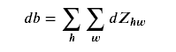
db[:,:,:,c] += dZ[i, h, w, c]
dA_prev[i, :, :, :] = dA_prev_pad[i, pad:-pad, pad:-pad, :]
### END CODE HERE ###
# Making sure your output shape is correct
assert(dA_prev.shape == (m, n_H_prev, n_W_prev, n_C_prev))
return dA_prev, dW, dbPooling layer - backward pass:
Max pooling - backward pass
在进入池化层的反向传播之前,构建一个名为create_mask_from_window()的辅助函数,它执行以下操作:
此函数创建一个“掩码”矩阵,用于跟踪矩阵的最大值。 True(1)表示X中最大值的位置,其他条目为False(0)。 会看到平均合并的后向传递将与此类似,但使用不同的掩码。
def create_mask_from_window(x):

    ### START CODE HERE ### (≈1 line)
    mask = (x == np.max(x))
    ### END CODE HERE ###

    return mask
注:为什么我们要记录最大的位置? 这是因为这是最终影响输出的输入值,因此也影响了成本。 Backprop正在计算与成本相关的梯度,因此影响最终成本的任何事物都应该具有非零梯度。 因此,backprop会将渐变“传播”回到影响成本的特定输入值。
Average pooling - backward pass
def distribute_value(dz, shape):
    ### START CODE HERE ###
    # Retrieve dimensions from shape (≈1 line)
    (n_H, n_W) = shape

    # Compute the value to distribute on the matrix (≈1 line)
    average = dz / (n_H * n_W)

    # Create a matrix where every entry is the "average" value (≈1 line)
    a = np.ones(shape) * average
    ### END CODE HERE ###

    return a
Putting it together: Pooling backward:
def pool_backward(dA, cache, mode = "max"):
    ### START CODE HERE ###
    # Retrieve information from cache (≈1 line)
    (A_prev, hparameters) = cache

    # Retrieve hyperparameters from "hparameters" (≈2 lines)
    stride = hparameters['stride']
    f = hparameters['f']

    # Retrieve dimensions from A_prev's shape and dA's shape (≈2 lines)
    m, n_H_prev, n_W_prev, n_C_prev = A_prev.shape
    m, n_H, n_W, n_C = dA.shape

    # Initialize dA_prev with zeros (≈1 line)
    dA_prev = np.zeros_like(A_prev)

    for i in range(m):
        # select training example from A_prev (≈1 line)
        a_prev = A_prev[i]

        for h in range(n_H):                   # loop on the vertical axis
            for w in range(n_W):               # loop on the horizontal axis
                for c in range(n_C):           # loop over the channels (depth)

                    # Find the corners of the current "slice" (≈4 lines)
                    vert_start = h * stride
                    vert_end = vert_start + f
                    horiz_start = w * stride
                    horiz_end = horiz_start + f

                    # Compute the backward propagation in both modes.
                    if mode == "max":
                        a_prev_slice = a_prev[vert_start:vert_end, horiz_start:horiz_end, c]
                        # Create the mask from a_prev_slice (≈1 line)
                        mask = create_mask_from_window(a_prev_slice)
                        dA_prev[i, vert_start: vert_end, horiz_start: horiz_end, c] += mask * dA[i, vert_start, horiz_start, c]

                    elif mode == "average":
                        # Get the value a from dA (≈1 line)
                        da = dA[i, vert_start, horiz_start, c]
                        # Define the shape of the filter as fxf (≈1 line)
                        shape = (f, f)
                        dA_prev[i, vert_start: vert_end, horiz_start: horiz_end, c] += distribute_value(da, shape)

    ### END CODE ###

    # Making sure your output shape is correct
    assert(dA_prev.shape == A_prev.shape)

    return dA_prev
以上就是卷积神经网络的全部过程已经代码实现,下面贴上一个完整的卷积神经网络的例子,因为源码运行源码是训练的准确率以及测试集准确率都很低,所以开始尝试改变了学习率以及epoch次数。
import math
import numpy as np
import h5py
import matplotlib.pyplot as plt
import scipy
from PIL import Image
from scipy import ndimage
import tensorflow as tf
from tensorflow.python.framework import ops
from cnn_utils import *

np.random.seed(1)

X_train_orig, Y_train_orig, X_test_orig, Y_test_orig, classes = load_dataset()

X_train = X_train_orig/255.
X_test = X_test_orig/255.
Y_train = convert_to_one_hot(Y_train_orig, 6).T
Y_test = convert_to_one_hot(Y_test_orig, 6).T

def create_placeholders(n_H0, n_W0, n_C0, n_y):
    X = tf.placeholder(tf.float32, shape=[None, n_H0, n_W0, n_C0])
    Y = tf.placeholder(tf.float32, shape=[None, n_y])
    return X, Y


def initialize_parameters():

    tf.set_random_seed(1)

    ### START CODE HERE ### (approx. 2 lines of code)
    W1 = tf.get_variable(name='W1', dtype=tf.float32, shape=(4, 4, 3, 8), initializer=tf.contrib.layers.xavier_initializer(seed = 0))
    W2 = tf.get_variable(name='W2', dtype=tf.float32, shape=(2, 2, 8, 16), initializer=tf.contrib.layers.xavier_initializer(seed = 0))
    ### END CODE HERE ###

    parameters = {"W1": W1,
                  "W2": W2}                    #第1、2个卷积网络,第1个为3层对应RGB,第2个
                                               #为8层对应第1个卷积层网络的个数
    return parameters

'''
tf.reset_default_graph()                       #用于清除默认图形堆栈并重置全局默认图形
with tf.Session() as sess_test:                #首先对所有变量进行初始化,防止带有之前执行过程中的残留值
    parameters = initialize_parameters()
    init = tf.global_variables_initializer()   #开始训练前对变量进行初始化
    sess_test.run(init)                        #在Sess中启用模型并初始化变量
    print("W1 = " + str(parameters["W1"].eval()[1,1,1]))
    print("W2 = " + str(parameters["W2"].eval()[1,1,1]))
'''

# GRADED FUNCTION: forward_propagation

def forward_propagation(X, parameters):

    # Retrieve the parameters from the dictionary "parameters"
    W1 = parameters['W1']
    W2 = parameters['W2']

    Z1 = tf.nn.conv2d(input=X, filter=W1, strides=[1, 1, 1, 1], padding='SAME')
    # RELU
    A1 = tf.nn.relu(Z1)
    # MAXPOOL: window 8x8, sride 8, padding 'SAME'
    P1 = tf.nn.max_pool(value=A1, ksize=[1, 8, 8, 1], strides=[1, 8, 8, 1], padding='SAME')
    # CONV2D: filters W2, stride 1, padding 'SAME'
    Z2 = tf.nn.conv2d(input=P1, filter=W2, strides=[1, 1, 1, 1], padding='SAME')
    # RELU
    A2 = tf.nn.relu(Z2)
    # MAXPOOL: window 4x4, stride 4, padding 'SAME'
    P2 = tf.nn.max_pool(value=A2, ksize=[1, 4, 4, 1], strides=[1, 4, 4, 1], padding='SAME')
    # FLATTEN
    P = tf.contrib.layers.flatten(P2)
    # FULLY-CONNECTED without non-linear activation function (not not call softmax).
    # 6 neurons in output layer. Hint: one of the arguments should be "activation_fn=None"
    Z3 = tf.contrib.layers.fully_connected(P, 6, activation_fn=None)#没有激活函数
    ### END CODE HERE ###

    return Z3

'''
#前向传播的测试代码
tf.reset_default_graph()
with tf.Session() as sess:
    np.random.seed(1)
    X, Y = create_placeholders(64, 64, 3, 6)#n_H0, n_W0,initialize_parameters n_C0, n_y
    parameters = initialize_parameters()#初始化W参数
    Z3 = forward_propagation(X, parameters)
    init = tf.global_variables_initializer()
    sess.run(init)    #这里已经初始化参数W了
    a = sess.run(Z3, {X: np.random.randn(2,64,64,3)})  #, Y: np.random.randn(2,6)})  这里需要fetch参数X,Y并不需要用到
    print("Z3 = " + str(a))
'''

def compute_cost(Z3, Y):
    """
    Computes the cost
    Arguments:
    Z3 -- output of forward propagation (output of the last LINEAR unit), of shape (6, number of examples)
    Y -- "true" labels vector placeholder, same shape as Z3
    Returns:
    cost - Tensor of the cost function
    """
    cost = tf.reduce_mean(tf.nn.softmax_cross_entropy_with_logits_v2(logits=Z3, labels=Y))#计算总的lost
    return cost

'''
tf.reset_default_graph()
with tf.Session() as sess:
    np.random.seed(1)
    X, Y = create_placeholders(64, 64, 3, 6)
    parameters = initialize_parameters()
    Z3 = forward_propagation(X, parameters)
    cost = compute_cost(Z3, Y)
    init = tf.global_variables_initializer()
    sess.run(init)
    a = sess.run(cost, {X: np.random.randn(4,64,64,3), Y: np.random.randn(4,6)})
    print("cost = " + str(a))
'''

def model(X_train, Y_train, X_test, Y_test, learning_rate = 0.01,
          num_epochs = 200, minibatch_size = 64, print_cost = True):
    """
    Implements a three-layer ConvNet in Tensorflow:
    CONV2D -> RELU -> MAXPOOL -> CONV2D -> RELU -> MAXPOOL -> FLATTEN -> FULLYCONNECTED
    Arguments:
    X_train -- training set, of shape (None, 64, 64, 3)
    Y_train -- test set, of shape (None, n_y = 6)
    X_test -- training set, of shape (None, 64, 64, 3)
    Y_test -- test set, of shape (None, n_y = 6)
    learning_rate -- learning rate of the optimization
    num_epochs -- number of epochs of the optimization loop
    minibatch_size -- size of a minibatch
    print_cost -- True to print the cost every 100 epochs
    Returns:
    train_accuracy -- real number, accuracy on the train set (X_train)
    test_accuracy -- real number, testing accuracy on the test set (X_test)
    parameters -- parameters learnt by the model. They can then be used to predict.
    """

    ops.reset_default_graph()                         # to be able to rerun the model without overwriting tf variables
    tf.set_random_seed(1)                             # to keep results consistent (tensorflow seed)
    seed = 3                                          # to keep results consistent (numpy seed)
    (m, n_H0, n_W0, n_C0) = X_train.shape
    n_y = Y_train.shape[1]
    costs = []                                        # To keep track of the cost

    X, Y = create_placeholders(n_H0, n_W0, n_C0, n_y)
    parameters = initialize_parameters()

    Z3 = forward_propagation(X, parameters)  #占位

    cost = compute_cost(Z3, Y)

    optimizer = tf.train.AdamOptimizer(learning_rate).minimize(cost)

    init = tf.global_variables_initializer()

    with tf.Session() as sess:

        sess.run(init)
        for epoch in range(num_epochs):
            minibatch_cost = 0.
            num_minibatches = int(m / minibatch_size) # number of minibatches of size minibatch_size in the train set
            #seed = seed + 1
            minibatches = random_mini_batches(X_train, Y_train, minibatch_size, seed) #每迭代一次搅一次

            for minibatch in minibatches:           #舍弃最后不足64个样本的mini_batch
                (minibatch_X, minibatch_Y) = minibatch
                # IMPORTANT: The line that runs the graph on a minibatch.
                _ , temp_cost = sess.run([optimizer, cost], feed_dict={X: minibatch_X, Y: minibatch_Y})

                minibatch_cost += temp_cost / num_minibatches  #取均值


            # Print the cost every epoch
            if print_cost == True and epoch % 10 == 0:
                print ("Cost after epoch %i: %f" % (epoch, minibatch_cost))
                data=open("test.txt",'a')
                print ("Cost after epoch %i: %f" % (epoch, minibatch_cost),file=data)
                data.close()
            if print_cost == True and epoch % 1 == 0:       #每一个minibatch_cost都记录
                costs.append(minibatch_cost)


        # plot the cost
        plt.plot(np.squeeze(costs))  #costs由for而来,因此x轴默认为epoch
        plt.ylabel('cost')
        plt.xlabel('iterations (per tens)')
        plt.title("Learning rate =" + str(learning_rate))
        plt.show()

        # Calculate the correct predictions
        predict_op = tf.argmax(Z3, 1)
        # 返回的是Z3中的最大值的索引号,如果vector是一个向量,那就返回一个值,如果是一个矩阵,那就返回一个向量,这个向量的每一个维度都是相对应矩阵行的最大值元素的索引号。
        correct_prediction = tf.equal(predict_op, tf.argmax(Y, 1))

        # Calculate accuracy on the test set
        accuracy = tf.reduce_mean(tf.cast(correct_prediction, "float"))  #转换为浮点数后求均值
        print(accuracy)
        train_accuracy = accuracy.eval({X: X_train, Y: Y_train})
        test_accuracy = accuracy.eval({X: X_test, Y: Y_test})
        # 和最主要的区别就在于你可以使用sess.run()在同一步获取多个tensor中的值
        print("Train Accuracy:", train_accuracy)
        print("Test Accuracy:", test_accuracy)

        return train_accuracy, test_accuracy, parameters

_, _, parameters = model(X_train, Y_train, X_test, Y_test)
运行结果:
Cost after epoch 0: 1.919799
Cost after epoch 10: 1.033018
Cost after epoch 20: 0.552845
Cost after epoch 30: 0.390024
Cost after epoch 40: 0.477188
Cost after epoch 50: 0.252454
Cost after epoch 60: 0.214543
Cost after epoch 70: 0.173962
Cost after epoch 80: 0.168894
Cost after epoch 90: 0.182265
Cost after epoch 100: 0.195930
Cost after epoch 110: 0.127377
Cost after epoch 120: 0.097412
Cost after epoch 130: 0.097927
Cost after epoch 140: 0.114083
Cost after epoch 150: 0.135697
Cost after epoch 160: 0.190367
Cost after epoch 170: 0.079545
Cost after epoch 180: 0.093178
Cost after epoch 190: 0.150684

第30次epoch时损失突然变大,然后随后就下降了,最后一段也出现的这种情况。最佳结果出现在130次epoch时,通过分析得知出现这种情况的原因是因为之前学习率过小,收敛速度慢,所以增大了学习率,导致训练不稳定,甚至导致发散。一般来说,我们会设置学习率衰减,一开始用稍微大一点的学习率,让收敛快一些,等差不多收敛了,把学习率降低,这样可以防止摇摆。
下面加上几段代码实现,网络自动更新学习率。
全连接层: