One-Shot Visual Imitation Learning via Meta-Learning

版权声明：Copyright reserved to Hazekiah Wang ([email protected]) https://blog.csdn.net/u010909964/article/details/84501919

Introduction

The goal of this work is to enable a robotic generalist to only learn from very few demonstrations, which may even be raw videos. This problem setting instantly brings us into the setting of one-shot (few data) visual imitation learning (learn from demos).

The paper mentions two major challenge of imitation learning: 1) compounding errors (which is not settled in this work), and 2) plenty of data. Prior efforts in reducing data resort to Inverse RL which can infer the reward function from a few demos. Here the author starts from meta-learning which compensates the lack of data via reusing experiences learned from similar (transferable, if more accurately speaking) tasks.

So in the background of meta-learning, the problem is re-formulated as how to effectively learn a policy (from meta-train tasks) that can quickly adapt to new tasks (meta-test tasks). Quick learning is required because we have only very few samples (demos of course).

MAML for imitation learning

Suppose we have a lot of tasks obeying a task distribution $P(T)$, where each task is defined by a triplet of (expert demonstrations, loss function, task description) that follows the setting of imitation learning.
Meta-train dataset is composed of sampled tasks used for meta-learning, meta-test dataset is one for evaluating the model’s adaptability performance.

MAML (Model-Agnostic Meta-Learning) is straight-forward if I interpret it as finding such policy parameters that (will) achieve maximal overall performance after its normal gradient update for each meta-train task specific to the task’s loss function.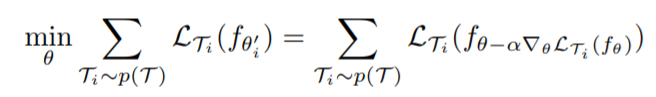
This is exactly following the raw intent of fast adapt for new tasks, as the objective function itself represents an expectation of performance across meta-train tasks, and we update parameters with its gradients, indicating that the objective is being pursued.

To break this approach apart more precisely (and clearly), there are actually three steps: 1) disguise we perform fast adapt to some unknown tasks, 2) sum over the performance of theses imaginary fast adapted solutions, 3) optimize this overall performance to find the (optimal) starting point from which to begin fast adapt.

Notice there are two gradient update step in the approach, one for the inner loss, another for the outer. As this is what meta-learning process composes, at least two samples is needed for the update. So in the meta-train dataset, each task should be equipped with at least two demonstrations.

Besides, although the original problem setting is claiming to input only raw videos - which refers to the testing stage (meta-test) indeed - this is not true for meta-train dataset. I think it would be safer to let the robot to at least experience what the standard actions should be, instead of somehow extracting those from raw videos that might well involve errors.

Q1

A messy point of MAML is that, we estimate the expected performance of fast adapt on the basis of the initial parameters, say $\theta_0$, and we optimize the objective on the basis of $\theta_0$ to $\theta_1$, then the fast adapt indeed performs upon $\theta_1$ instead of what we used to estimate and for optimization. Will this bias between $\theta_0$ and $\theta_1$ affects our performance estimate and further undermines the efficacy of the optimization?

At last I still want to make up a point about what exactly do we do during inference time. Actually training and inference is combined in this approach: 1) we first perform the meta-learning to get a pre-trained policy based on meta-train tasks, and 2) fine-tune to adapt the policy to the new task on hand.

Improvements

Two-head architecture

Suppose the architecture of the policy network is as simple as several conv layers followed by dense layers.

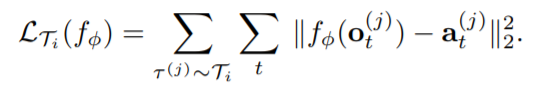
Remember previously we involve two loss function in the objective function, which are in essence the same function, using the supervised MSE loss between expert demonstrations and predicted action sequences. If we have the two loss function use different final dense layers, they are no longer the same.

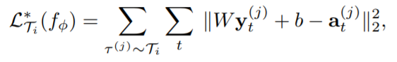
It follows that if we get rid of the ground truth expert demonstration term in the inner loss function, the network seems to be producing its own loss function.


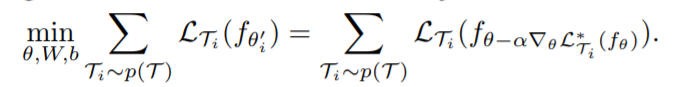
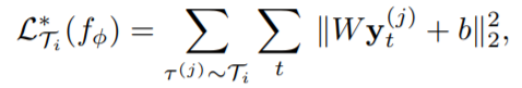
At first glance, I don’t think this formulation is valid, because how can we evaluate the expected performance of adaptability if ground truths is not even used? But then I realize it is the outer loss function that really inspects the performance of adapted polices, which does include the expert demonstrations. So getting rid of the ground truths in the inner loss function is just like handing in the control over the adaptability evaluation metrics to the network itself. Previously we believe the supervised MSE loss measures the goodness of a policy and hope the fast adapt will advance in this measure, now we just let our network to determine by itself how to meansure the goodness, with learned parameters in the final dense layers.

This modification provides convenience for demonstrations that include no actions but only observations, which is set as raw pixel inputs in the initial goal. To be more specific, during the testing stage, this learned loss function is set as the adapt objective function to fine-tune the pre-trained policy, so that raw videos are usable demonstrations.

Bias Transformation

The idea is to reparameterize the bias $b$ into $W_2z+b$, which is said to

… increases the representational power of the gradient, without affecting the representation power of the network itself.

The logics is :

1. if we write out the gradient of $L$ w.r.t $b$, we see that it is dependent on parameters in its prior layers,
2. but if we add the reparameterization with new parameter $z$, we find the gradient dependent on $W_2$ and $z$.

Q2

But I do not understand the benefits for this trick (maybe after I read through the experiment section).

Questions

1. Will $\theta_0$ asymptotically estimate $\theta_1$?
2. What exactly is the benefit of bias transformation?
3. I am not quite sure about my interpretation of the two head architecture.