Scikit learn Sample1—Isotonic Regression

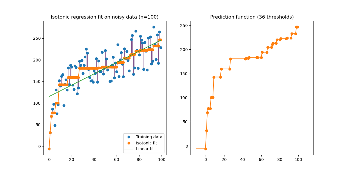
生成数据的等渗回归的图示。等张回归发现函数的非递减近似，同时最小化训练数据的均方误差。这种模型的好处是它不假设任何形式的目标函数，如线性。为了比较，还给出了线性回归。

print(__doc__)

# Author: Nelle Varoquaux <[email protected]>
#         Alexandre Gramfort <[email protected]>
# License: BSD

import numpy as np
import matplotlib.pyplot as plt
from matplotlib.collections import LineCollection

from sklearn.linear_model import LinearRegression
from sklearn.isotonic import IsotonicRegression
from sklearn.utils import check_random_state

n = 100
x = np.arange(n)
rs = check_random_state(0)
y = rs.randint(-50, 50, size=(n,)) + 50. * np.log1p(np.arange(n))

# #############################################################################
# Fit IsotonicRegression and LinearRegression models

ir = IsotonicRegression()

y_ = ir.fit_transform(x, y)

lr = LinearRegression()
lr.fit(x[:, np.newaxis], y)  # x needs to be 2d for LinearRegression

# #############################################################################
# Plot result

segments = [[[i, y[i]], [i, y_[i]]] for i in range(n)]
lc = LineCollection(segments, zorder=0)
lc.set_array(np.ones(len(y)))
lc.set_linewidths(np.full(n, 0.5))

fig = plt.figure()
plt.plot(x, y, 'r.', markersize=12)
plt.plot(x, y_, 'g.-', markersize=12)
plt.plot(x, lr.predict(x[:, np.newaxis]), 'b-')
plt.gca().add_collection(lc)
plt.legend(('Data', 'Isotonic Fit', 'Linear Fit'), loc='lower right')
plt.title('Isotonic regression')
plt.show()

注释：

   IsotonicRegression： 

min sum w_i (y[i] - y_[i]) ** 2

subject to y_[i] <= y_[j] whenever X[i] <= X[j]
and min(y_) = y_min, max(y_) = y_max

where:

• y[i] are inputs (real numbers)
• y_[i] are fitted
• X specifies the order. If X is non-decreasing then y_ is non-decreasing.
• w[i] are optional strictly positive weights (default to 1.0)
• y [i]是输入（实数）
• y_ [i]拟合X指定顺序。
• 如果X不递减，则y_不递减。
• w [i]是可选的严格正权重（默认为1.0）

Linear Regression：

>>> import numpy as np
>>> from sklearn.linear_model import LinearRegression
>>> X = np.array([[1, 1], [1, 2], [2, 2], [2, 3]])
>>> # y = 1 * x_0 + 2 * x_1 + 3
>>> y = np.dot(X, np.array([1, 2])) + 3
>>> reg = LinearRegression().fit(X, y)
>>> reg.score(X, y)
1.0
>>> reg.coef_
array([1., 2.])
>>> reg.intercept_ 
3.0000...
>>> reg.predict(np.array([[3, 5]]))
array([16.])