EM算法：从极大似然估计导出EM算法（还算通俗易懂）

之前看了《统计学习方法》，吴恩达老师的cs229讲义，一起看感觉很昏（如果要看建议选择其中一个，《统计学习方法》里面基本很少会写到 $y_i$ 而都是用 $Y$ 只用了极大化没有写出我们熟悉的似然函数？！，cs229有视频，但我喜欢看书），网上看了点博客大部分好像也是来自cs229讲义。这里结合七月里面一个博士讲的与自己的理解来写出从极大似然估计推出EM算法好了。

1、隐变量与概率模型参数

EM算法：概率模型有时既含有观测变量，又含有隐变量。如果概率模型的变量都是观测变量，那么给定数据，就可以直接使用极大似然估计来求得参数或者贝叶斯估计模型参数。但是如果变量中有因变量，那么这些方法就不行了，这个时候就可以使用EM算法，EM算法就是含有隐变量的概率模型参数的极大似然估计方法。

下面给出《统计学习方法》中的例子

在这里插入图片描述

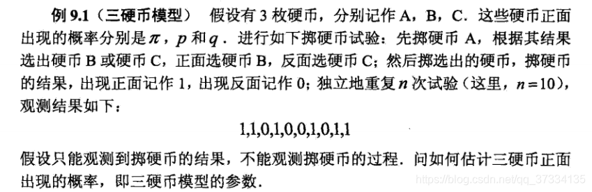
观测结果 ${1,1,0,1,0,0,1,0,1,1}$ 我们用变量 $Y$ 表示，叫做显变量，这里取值是0或1

而掷的硬币A的结果我们是不知道的，我们用变量 $Z$ 表示，叫做隐变量

2、EM算法推导

而 $\pi，p，q$ 则是模型参数，现在我们要求这三个参数。由于是改了模型，我们知道观测结果来求参数，自然想到使用极大似然估计。根据极大似然估计定义，概率分布 $P(Y=y_i)=p_\theta(y_i;)$ ，其中 $\theta$ 为模型参数

先回顾下概率公式（推导会用到）：
$p(y)=\sum\limits_{z}p(z)p(y|z)=\sum\limits_{z}p(y,z)$ 全概率公式和贝叶斯公式
$\sum\limits_{z}p(z|y)=1$

写出极大似然函数

$L(\theta)=\prod\limits_{i=1}^{n}p_\theta(y_i)\\=\prod\limits_{i=1}^{n}\sum\limits_{z}p_\theta(y_i,z)\\=\prod\limits_{i=1}^{n}\sum\limits_{z}p_\theta(z)p_\theta(y_i|z)$

写出对数形式

扫描二维码关注公众号，回复： 4899897 查看本文章

$l(\theta)=lnL(\theta)=ln\prod\limits_{i=1}^{n}\sum\limits_{z}p_\theta(z)p_\theta(y_i|z)=\sum\limits_{i=1}^{n}ln[\sum\limits_{z}p_\theta(z)p_\theta(y_i|z)]$

通常到这里就要对参数求导 $\theta$ 求导从而得到似然函数的极大值，但是这里由于对数里面存在求和，这种情况是难以求解的。这种情况下，通常的做法是使用迭代逐步去毕竟最优解，而EM算法就是这样一种迭代算法，假设第 $n$ 次迭代求出的参数为 $\theta_n$ ，我们希望下一次迭代得到的参数满足 $l(\theta_{n+1})>l(\theta_{n})$

$l(\theta)-l(\theta_n)=\sum\limits_{i=1}^{n}(ln\sum\limits_{z}p_\theta(z)p_\theta(y_i|z)-ln^{p_{\theta_n}(y_i))}$

对 $p_\theta(z)p_\theta(y_i|z)$ 进行乘一项除一项得到 $p_{\theta_n}(z|y_i)\frac{p_\theta(z)p_\theta(y_i|z)}{p_{\theta_n}(z|y_i)}$

$l(\theta)-l(\theta_n)=\sum\limits_{i=1}^{n}(ln\sum\limits_{z}p_{\theta_n}(z|y_i)\frac{p_\theta(z)p_\theta(y_i|z)}{p_{\theta_n}(z|y_i)}-ln^{p_{\theta_n}(y_i)})$

由于 $\sum\limits_{z}p(z|y)=1$ ，所以 $ln^{p_{\theta_n}(y_i)}=\sum\limits_{z}ln^{p_{\theta_n}(y_i)}p_{\theta_n}(z|y_i)$

$l(\theta)-l(\theta_n)=\sum\limits_{i=1}^{n}(ln\sum\limits_{z}p_{\theta_n}(z|y_i)\frac{p_\theta(z)p_\theta(y_i|z)}{p_{\theta_n}(z|y_i)}-\sum\limits_{z}ln^{p_{\theta_n}(y_i)}p_{\theta_n}(z|y_i))$

下面介绍下琴生不等式(Jensen)

看下面的图，曲线对应的是一个凹函数
在这里插入图片描述

对于凸函数，上面的符号改成小于等于即可，可以自己画图。

$ln\sum\limits_{z}p_{\theta_n}(z|y_i)\frac{p_\theta(z)p_\theta(y_i|z)}{p_{\theta_n}(z|y_i)}\geq \sum\limits_{z}p_{\theta_n}(z|y_i)ln^{\frac{p_\theta(z)p_\theta(y_i|z)}{p_{\theta_n}(z|y_i)}}$

$=>l(\theta)-l(\theta_n)\geq \sum\limits_{i=1}^{n}(\sum\limits_{z}p_{\theta_n}(z|y_i)ln^{\frac{p_\theta(z)p_\theta(y_i|z)}{p_{\theta_n}(z|y_i)}}-\sum\limits_{z}ln^{p_{\theta_n}(y_i)}p_{\theta_n}(z|y_i))= \sum\limits_{i=1}^{n} \sum\limits_{z}(p_{\theta_n}(z|y_i)ln^{{\frac{p_\theta(z)p_\theta(y_i|z)}{p_{\theta_n}(y_i)p_{\theta_n}(z|y_i)}}})$

最后我们得到

$l(\theta)\geq l(\theta_n)+ \sum\limits_{i=1}^{n} \sum\limits_{z}(p_{\theta_n}(z|y_i)ln^{{\frac{p_\theta(z)p_\theta(y_i|z)}{p_{\theta_n}(y_i)p_{\theta_n}(z|y_i)}}})$

记 $B(\theta|\theta_n)= l(\theta_n)+ \sum\limits_{i=1}^{n} \sum\limits_{z}(p_{\theta_n}(z|y_i)ln^{{\frac{p_\theta(z)p_\theta(y_i|z)}{p_{\theta_n}(y_i)p_{\theta_n}(z|y_i)}}})$ ，那么 $l(\theta)\geq B(\theta|\theta_n)$

称 $B(\theta|\theta_n)$ 为 $l(\theta)的下边界函数$ ，可以注意到:
$B(\theta_n|\theta_n)=l(\theta_n)+ \sum\limits_{i=1}^{n} \sum\limits_{z}(p_{\theta_n}(z|y_i)ln^{{\frac{p_{\theta_n}(z)p_{\theta_n}(y_i|z)}{p_{\theta_n}(y_i)p_{\theta_n}(z|y_i)}}})=l(\theta_n)$

只要我们最大化 $B(\theta|\theta_n)$ 那么 $l(\theta)$ 也就可以尽可能大。再来看 $B(\theta|\theta_n)$ ，我们要求他的极大值

$B(\theta|\theta_n)= l(\theta_n)+ \sum\limits_{i=1}^{n} \sum\limits_{z}(p_{\theta_n}(z|y_i)ln^{\frac{p_\theta(z)p_\theta(y_i|z)}{p_{\theta_n}(y_i)p_{\theta_n}(z|y_i)}})\\= l(\theta_n)+ \sum\limits_{i=1}^{n} \sum\limits_{z}p_{\theta_n}(z|y_i)ln^{p_\theta(z)p_\theta(y_i|z)}-\sum\limits_{i=1}^{n} \sum\limits_{z}p_{\theta_n}(z|y_i)ln^{p_{\theta_n}(y_i)p_{\theta_n}(z|y_i)}$

去掉常数项，得到仅与 $\theta$ 有关的项 $\sum\limits_{i=1}^{n} \sum\limits_{z}p_{\theta_n}(z|y_i)ln^{p_\theta(z)p_\theta(y_i|z)}=\sum\limits_{i=1}^{n} \sum\limits_{z}p_{\theta_n}(z|y_i)ln^{p_\theta(y_i,z)}$ ，在这里称 $Q(\theta|\theta_n)=\sum\limits_{i=1}^{n} \sum\limits_{z}p_{\theta_n}(z|y_i)ln^{p_\theta(y_i,z)}$ 为 $Q$ 函数（《统计学习方法》中没有直接写最外层的求和，所以写的是 $\sum\limits_{z}p_{\theta_n}(z|y_i)ln^{p_\theta(y_i,z)}$ ）以后进行求导即可。这样我们就得到了第 $n+1$ 步的参数值 $\theta_{n+1}$

$\theta_{n+1}=\arg\max\limits_{\theta}Q(\theta|\theta_n)$

第 $n+2$ 步， $n+3$ 步，一直这样往下求，直到收敛，比如 $||\theta_{n+1}-\theta_n||<\varepsilon$ 。

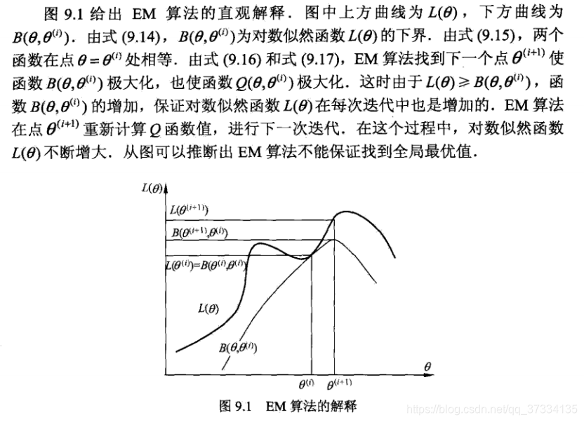
下面给出《统计学习方法》中的直观解释：

在这里插入图片描述

3、EM算法过程

到这里我们引出EM算法步骤：

输入：观测数据 $Y$ ，联合分布 $P(Y,Z;\theta)$ ，条件分布 $P(Z|Y;\theta)$
输出：模型参数 $\theta$

（1）、选择参数的初始值 $\theta_0$ 开始进行迭代；
（2）、E（Expection）步：记第n次迭代参数为 $\theta_n$ ，那么计算 $n+1$ 次的E步

$Q(\theta|\theta_n)=\sum\limits_{i=1}^{n} \sum\limits_{z}p_{\theta_n}(z|y_i)ln^{p_\theta(y_i,z)}$

（3）、M（Maximization）步：求使得 $Q(\theta|\theta_n)$ 最大化的 $\theta_{n+1}$ ，即确定第 $n+1$ 次的模型参数

$\theta_{n+1}=\arg\max\limits_{\theta}Q(\theta|\theta_n)$

（4）、重复（2），（3）直到收敛。

注意：初值选的不一样，结果可能不一样，EM算法对初值是敏感的。