天池 O2O 优惠券使用预测思路解析与代码实战

版权声明：本文为博主原创文章，未经博主允许不得转载。 https://blog.csdn.net/red_stone1/article/details/83859845

个人网站：redstonewill.com

前阵子因为机器学习训练营的任务安排，需要打一场 AI 比赛。然后就了解到最近热度很高且非常适合新人入门的一场比赛：天池新人实战赛o2o优惠券使用预测。今天，红色石头把这场比赛的一些初级理论分析和代码实操分享给大家。本文会讲解的很细，目的是带领大家走一遍比赛流程，实现机器学习理论分析到比赛实战的进阶。话不多说，我们开始吧！

比赛介绍

首先附上这场比赛的链接：

https://tianchi.aliyun.com/getStart/introduction.htm?spm=5176.100066.0.0.518433afBqXIKM&raceId=231593

本赛题的比赛背景是随着移动设备的完善和普及，移动互联网+各行各业进入了高速发展阶段，这其中以 O2O（Online to Offline）消费最为吸引眼球。本次大赛为参赛选手提供了 O2O 场景相关的丰富数据，希望参赛选手通过分析建模，精准预测用户是否会在规定时间（15 天）内使用相应优惠券。

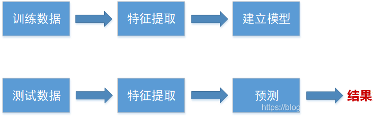
从机器学习模型的角度来说，这是一个典型的分类问题，其过程就是根据已有训练集进行训练，得到的模型再对测试进行测试并分类。整个过程如下图所示：

评估方式

我们知道评估一个机器学习模型有多种方式，最常见的例如准确率（Accuracy）、精确率（Precision）、召回率（Recall）。一般使用精确率和召回率结合的方式 F1 score 能较好地评估模型性能（特别是在正负样本不平衡的情况下）。而在本赛题，官方规定的评估方式是 AUC，即 ROC 曲线与横坐标围成的面积。如下图所示：

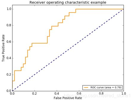
关于 ROC 和 AUC 的概念这里不加解释，至于为什么要使用 ROC 和 AUC 呢？因为 ROC 曲线有个很好的特性：当测试集中的正负样本的分布变化的时候，ROC曲线能够保持不变。也就是说能够更好地处理正负样本分布不均的场景。

数据集导入

对任何机器学习模型来说，数据集永远是最重要的。接下来，我们就来看看这个比赛的数据集是什么样的。

首先来看一下大赛提供给我们的数据集：

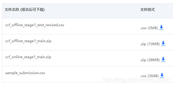
总共有四个文件，分别是：

• ccf_offline_stage1_test_revised.csv

• ccf_offline_stage1_train.csv

• ccf_online_stage1_train.csv

• sample_submission.csv

其中，第 2 个是线下训练集，第 1 个是线下测试集，第 3 个是线上训练集（本文不会用到），第 4 个是预测结果提交到官网的文件格式（需按照此格式提交才有效）。也就是说我们使用第 2 个文件来训练模型，对第 1 个文件进行预测，得到用户在 15 天内使用优惠券的概率值。

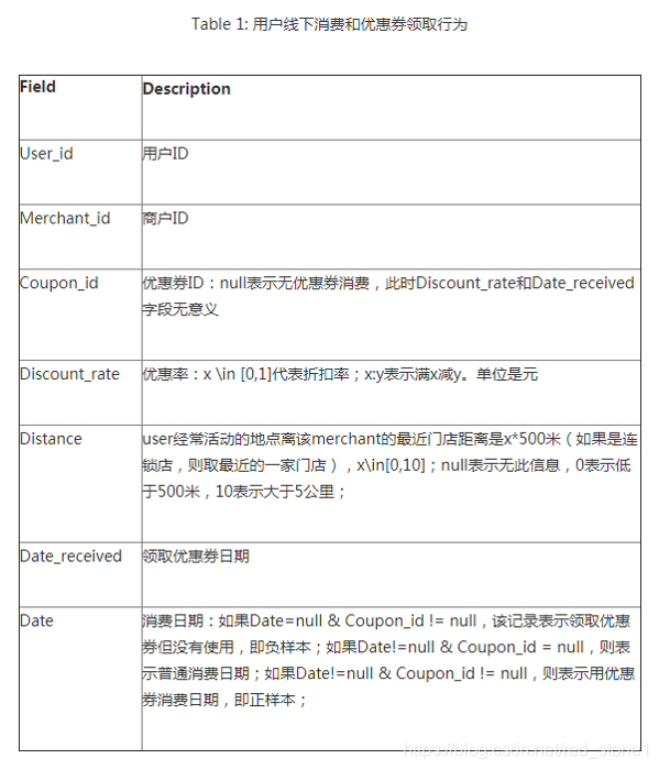
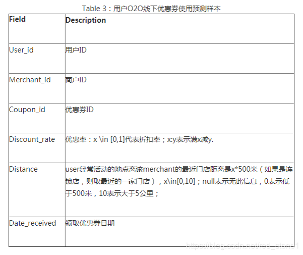
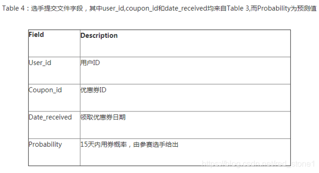
接下来，对 2、1、4 文件中字段进行列举，字段解释如下图所示。

ccf_offline_stage1_train.csv：

ccf_offline_stage1_test_revised.csv：

sample_submission.csv：

重点记住两个字段：Date_received 是领取优惠券日期，Date 是消费日期。待会我将详细介绍。

介绍完几个数据文件和字段之后，我们就来编写程序，导入训练集和测试集，同时导入需要用到的库。

# import libraries necessary for this project
import os, sys, pickle

import numpy as np
import pandas as pd

from datetime import date

from sklearn.model_selection import KFold, train_test_split, StratifiedKFold, cross_val_score, GridSearchCV
from sklearn.pipeline import Pipeline
from sklearn.linear_model import SGDClassifier, LogisticRegression
from sklearn.preprocessing import StandardScaler
from sklearn.metrics import log_loss, roc_auc_score, auc, roc_curve
from sklearn.preprocessing import MinMaxScaler

# display for this notebook
%matplotlib inline
%config InlineBackend.figure_format = 'retina'

导入数据：

dfoff = pd.read_csv('data/ccf_offline_stage1_train.csv')
dfon = pd.read_csv('data/ccf_online_stage1_train.csv')
dftest = pd.read_csv('data/ccf_offline_stage1_test_revised.csv')

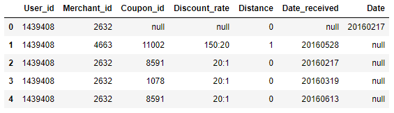
dfoff.head(5)

是训练集前 5 行显示如下：

接下来，我们来做个简单统计，看一看究竟用户是否使用优惠券消费的情况。

print('有优惠卷，购买商品：%d' % dfoff[(dfoff['Date_received'] != 'null') & (dfoff['Date'] != 'null')].shape[0])
print('有优惠卷，未购商品：%d' % dfoff[(dfoff['Date_received'] != 'null') & (dfoff['Date'] == 'null')].shape[0])
print('无优惠卷，购买商品：%d' % dfoff[(dfoff['Date_received'] == 'null') & (dfoff['Date'] != 'null')].shape[0])
print('无优惠卷，未购商品：%d' % dfoff[(dfoff['Date_received'] == 'null') & (dfoff['Date'] == 'null')].shape[0])

有优惠卷，购买商品：75382
有优惠卷，未购商品：977900
无优惠卷，购买商品：701602
无优惠卷，未购商品：0

可见，很多人（701602）购买商品却没有使用优惠券，也有很多人（977900）有优惠券但却没有使用，真正使用优惠券购买商品的人（75382）很少！所以，这个比赛的意义就是把优惠券送给真正可能会购买商品的人。

特征提取

毫不夸张第说，构建机器学习模型，特征工程可能比选择哪种算法更加重要。接下来，我们就来研究一下哪些特征可能对模型训练有用。

1.打折率（Discount_rate）

首先，第一个想到的特征应该是优惠卷的打折率。因为很显然，一般情况下优惠得越多，用户就越有可能使用优惠券。那么，我们就来看一下训练集中优惠卷有哪些类型。

print('Discount_rate 类型：\n',dfoff['Discount_rate'].unique())

Discount_rate 类型：
[‘null’ ‘150:20’ ‘20:1’ ‘200:20’ ‘30:5’ ‘50:10’ ‘10:5’ ‘100:10’ ‘200:30’ ‘20:5’ >‘30:10’ ‘50:5’ ‘150:10’ ‘100:30’ ‘200:50’ ‘100:50’ ‘300:30’ ‘50:20’ ‘0.9’ ‘10:1’ >‘30:1’ ‘0.95’ ‘100:5’ ‘5:1’ ‘100:20’ ‘0.8’ ‘50:1’ ‘200:10’ ‘300:20’ ‘100:1’ >‘150:30’ ‘300:50’ ‘20:10’ ‘0.85’ ‘0.6’ ‘150:50’ ‘0.75’ ‘0.5’ ‘200:5’ ‘0.7’ >‘30:20’ ‘300:10’ ‘0.2’ ‘50:30’ ‘200:100’ ‘150:5’]

根据打印的结果来看，打折率分为 3 种情况：

• ‘null’ 表示没有打折

• [0,1] 表示折扣率

• x:y 表示满 x 减 y

那我们的处理方式可以构建 4 个函数，分别提取 4 种特征，分别是：

• 打折类型：getDiscountType()

• 折扣率：convertRate()

• 满多少：getDiscountMan()

• 减多少：getDiscountJian()

函数代码如下：

# Convert Discount_rate and Distance
def getDiscountType(row):
   if row == 'null':
       return 'null'
   elif ':' in row:
       return 1
   else:
       return 0

def convertRate(row):
   """Convert discount to rate"""
   if row == 'null':
       return 1.0
   elif ':' in row:
       rows = row.split(':')
       return 1.0 - float(rows[1])/float(rows[0])
   else:
       return float(row)
   
def getDiscountMan(row):
   if ':' in row:
       rows = row.split(':')
       return int(rows[0])
   else:
       return 0

def getDiscountJian(row):
   if ':' in row:
       rows = row.split(':')
       return int(rows[1])
   else:
       return 0
   
def processData(df):
   
   # convert discount_rate
   df['discount_type'] = df['Discount_rate'].apply(getDiscountType)
   df['discount_rate'] = df['Discount_rate'].apply(convertRate)
   df['discount_man'] = df['Discount_rate'].apply(getDiscountMan)
   df['discount_jian'] = df['Discount_rate'].apply(getDiscountJian)
   
   print(df['discount_rate'].unique())
   
   return df

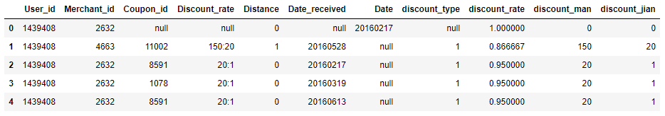
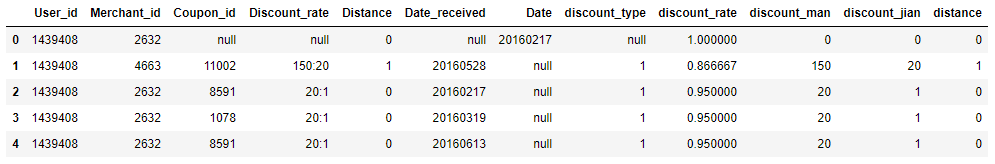
然后，对训练集和测试集分别进行进行 processData（）函数的处理：

dfoff = processData(dfoff)
dftest = processData(dftest)

处理之后，我们可以看到训练集和测试集都多出了 4 个新的特征：discount_type、discount_rate、discount_man、discount_jian。

2.距离（Distance）

距离字段表示用户与商店的地理距离，显然，距离的远近也会影响到优惠券的使用与否。那么，我们就可以把距离也作为一个特征。首先看一下距离有哪些特征值：

print('Distance 类型：',dfoff['Distance'].unique())

Distance 类型： [‘0’ ‘1’ ‘null’ ‘2’ ‘10’ ‘4’ ‘7’ ‘9’ ‘3’ ‘5’ ‘6’ ‘8’]

然后，定义提取距离特征的函数：

# convert distance
dfoff['distance'] = dfoff['Distance'].replace('null', -1).astype(int)
print(dfoff['distance'].unique())
dftest['distance'] = dftest['Distance'].replace('null', -1).astype(int)
print(dftest['distance'].unique())

处理之后，我们可以看到训练集和测试集都多出了 1 个新的特征：distance。

3.领劵日期（Date_received）

是还有一点很重要的是领券日期，因为一般而言，周末领取优惠券去消费的可能性更大一些。因此，我们可以构建关于领券日期的一些特征：

• weekday : {null, 1, 2, 3, 4, 5, 6, 7}

• weekday_type : {1, 0}（周六和周日为1，其他为0）

• Weekday_1 : {1, 0, 0, 0, 0, 0, 0}

• Weekday_2 : {0, 1, 0, 0, 0, 0, 0}

• Weekday_3 : {0, 0, 1, 0, 0, 0, 0}

• Weekday_4 : {0, 0, 0, 1, 0, 0, 0}

• Weekday_5 : {0, 0, 0, 0, 1, 0, 0}

• Weekday_6 : {0, 0, 0, 0, 0, 1, 0}

• Weekday_7 : {0, 0, 0, 0, 0, 0, 1}

其中用到了独热编码，让特征更加丰富。相应的这 9 个特征的提取函数为：

def getWeekday(row):
   if row == 'null':
       return row
   else:
       return date(int(row[0:4]), int(row[4:6]), int(row[6:8])).weekday() + 1

dfoff['weekday'] = dfoff['Date_received'].astype(str).apply(getWeekday)
dftest['weekday'] = dftest['Date_received'].astype(str).apply(getWeekday)

# weekday_type :  周六和周日为1，其他为0
dfoff['weekday_type'] = dfoff['weekday'].apply(lambda x: 1 if x in [6,7] else 0)
dftest['weekday_type'] = dftest['weekday'].apply(lambda x: 1 if x in [6,7] else 0)

# change weekday to one-hot encoding 
weekdaycols = ['weekday_' + str(i) for i in range(1,8)]
#print(weekdaycols)

tmpdf = pd.get_dummies(dfoff['weekday'].replace('null', np.nan))
tmpdf.columns = weekdaycols
dfoff[weekdaycols] = tmpdf

tmpdf = pd.get_dummies(dftest['weekday'].replace('null', np.nan))
tmpdf.columns = weekdaycols
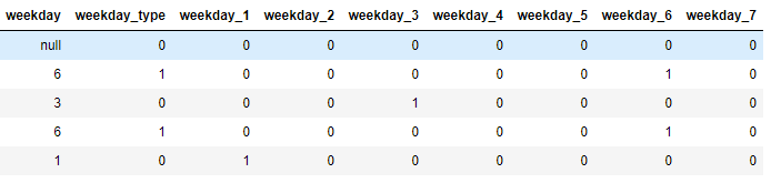
dftest[weekdaycols] = tmpdf

这样，我们就会在训练集和测试集上发现增加了 9 个关于领券日期的特征：

好了，经过以上简单的特征提取，我们总共得到了 14 个有用的特征：

• discount_rate

• discount_type

• discount_man

• discount_jian

• distance

• weekday

• weekday_type

• weekday_1

• weekday_2

• weekday_3

• weekday_4

• weekday_5

• weekday_6

• weekday_7

好了，我们的主要工作已经完成了大半！

标注标签 Label

有了特征之后，我们还需要对训练样本进行 label 标注，即确定哪些是正样本（y = 1），哪些是负样本（y = 0）。我们要预测的是用户在领取优惠券之后 15 之内的消费情况。所以，总共有三种情况：

1.Date_received == ‘null’：

表示没有领到优惠券，无需考虑，y = -1

2.(Date_received != ‘null’) & (Date != ‘null’) & (Date - Date_received <= 15)：

表示领取优惠券且在15天内使用，即正样本，y = 1

3.(Date_received != ‘null’) & ((Date == ‘null’) | (Date - Date_received > 15))：

表示领取优惠券未在在15天内使用，即负样本，y = 0

好了，知道规则之后，我们就可以定义标签备注函数了。

def label(row):
   if row['Date_received'] == 'null':
       return -1
   if row['Date'] != 'null':
       td = pd.to_datetime(row['Date'], format='%Y%m%d') - pd.to_datetime(row['Date_received'], format='%Y%m%d')
       if td <= pd.Timedelta(15, 'D'):
           return 1
   return 0

dfoff['label'] = dfoff.apply(label, axis=1)

我们可以使用这个函数对训练集进行标注，看一下正负样本究竟有多少：

print(dfoff['label'].value_counts())

0 988887
-1 701602
1 64395
Name: label, dtype: int64

很清晰地，正样本共有 64395 例，负样本共有 988887 例。显然，正负样本数量差别很大。这也是为什么会使用 AUC 作为模型性能评估标准的原因。

建立模型

接下来就是最主要的建立机器学习模型了。首先确定的是我们选择的特征是上面提取的 14 个特征，为了验证模型的性能，需要划分验证集进行模型验证，划分方式是按照领券日期，即训练集：20160101-20160515，验证集：20160516-20160615。我们采用的模型是简单的 SGDClassifier。

1.划分训练集和验证集

# data split
df = dfoff[dfoff['label'] != -1].copy()
train = df[(df['Date_received'] < '20160516')].copy()
valid = df[(df['Date_received'] >= '20160516') & (df['Date_received'] <= '20160615')].copy()
print('Train Set: \n', train['label'].value_counts())
print('Valid Set: \n', valid['label'].value_counts())

2.构建模型

def check_model(data, predictors):
   
   classifier = lambda: SGDClassifier(
       loss='log',  # loss function: logistic regression
       penalty='elasticnet', # L1 & L2
       fit_intercept=True,  # 是否存在截距，默认存在
       max_iter=100, 
       shuffle=True,  # Whether or not the training data should be shuffled after each epoch
       n_jobs=1, # The number of processors to use
       class_weight=None) # Weights associated with classes. If not given, all classes are supposed to have weight one.

   # 管道机制使得参数集在新数据集（比如测试集）上的重复使用，管道机制实现了对全部步骤的流式化封装和管理。
   model = Pipeline(steps=[
       ('ss', StandardScaler()), # transformer
       ('en', classifier())  # estimator
   ])

   parameters = {
       'en__alpha': [ 0.001, 0.01, 0.1],
       'en__l1_ratio': [ 0.001, 0.01, 0.1]
   }

   # StratifiedKFold用法类似Kfold，但是他是分层采样，确保训练集，测试集中各类别样本的比例与原始数据集中相同。
   folder = StratifiedKFold(n_splits=3, shuffle=True)
   
   # Exhaustive search over specified parameter values for an estimator.
   grid_search = GridSearchCV(
       model, 
       parameters, 
       cv=folder, 
       n_jobs=-1,  # -1 means using all processors
       verbose=1)
   grid_search = grid_search.fit(data[predictors], 
                                 data['label'])
   
   return grid_search

模型采用的是 SGDClassifier，使用了 Python 中的 Pipeline 管道机制，可以使参数集在新数据集（比如测试集）上的重复使用，管道机制实现了对全部步骤的流式化封装和管理。交叉验证采用 StratifiedKFold，其用法类似 Kfold，但是 StratifiedKFold 是分层采样，确保训练集，测试集中各类别样本的比例与原始数据集中相同。

3.训练

接下来就可以使用该模型对训练集进行训练了，整个训练过程大概 1-2 分钟的时间。

predictors = original_feature
model = check_model(train, predictors)

4.验证

然后对验证集中每个优惠券预测的结果计算 AUC，再对所有优惠券的 AUC 求平均。计算 AUC 的时候，如果 label 只有一类，就直接跳过，因为 AUC 无法计算。

# valid predict
y_valid_pred = model.predict_proba(valid[predictors])
valid1 = valid.copy()
valid1['pred_prob'] = y_valid_pred[:, 1]
valid1.head(5)

注意这里得到的结果 pred_prob 是概率值（预测样本属于正类的概率）。

最后，就可以对验证集计算 AUC。直接调用 sklearn 库自带的计算 AUC 函数即可。

# avgAUC calculation
vg = valid1.groupby(['Coupon_id'])
aucs = []
for i in vg:
   tmpdf = i[1] 
   if len(tmpdf['label'].unique()) != 2:
       continue
   fpr, tpr, thresholds = roc_curve(tmpdf['label'], tmpdf['pred_prob'], pos_label=1)
   aucs.append(auc(fpr, tpr))
print(np.average(aucs))

0.532344469452

最终得到的 AUC 就等于 0.53。

测试

训练完模型之后，就是使用训练好的模型对测试集进行测试了。并且将测试得到的结果（概率值）按照规定的格式保存成一个 .csv 文件。

# test prediction for submission
y_test_pred = model.predict_proba(dftest[predictors])
dftest1 = dftest[['User_id','Coupon_id','Date_received']].copy()
dftest1['Probability'] = y_test_pred[:,1]
dftest1.to_csv('submit.csv', index=False, header=False)
dftest1.head(5)

值得注意的是，这里得到的结果是概率值，最终的 AUC 是提交到官网之后平台计算的。因为测试集真正的 label 我们肯定是不知道的。

提交结果

好了，最后一步就是在比赛官网上提交我们的预测结果，即这里的 submit.csv 文件。提交完之后，过几个小时就可以看到成绩了。整个比赛的流程就完成了。

优化模型

其实，本文所述的整个比赛思路和算法是比较简单的，得到的结果和成绩也只能算是合格，名次不会很高。我们还可以运用各种手段优化模型，简单来说分为以下三种：

• 特征工程

• 机器学习

• 模型融合

总结

本文的主要目的是带领大家走一遍整个比赛的流程，培养一些比赛中特征提取和算法应用方面的知识。这个天池比赛目前还是比较火热的，虽然没有奖金，但是参赛人数已经超过 1.1w 了。看完本文之后，希望大家有时间去参加感受一下机器学习比赛的氛围，将理论应用到实战中去。

本文完整的代码我已经放在了 GitHub 上，有需要的请自行领取：

https://github.com/RedstoneWill/MachineLearningInAction-Camp/tree/master/Week4/o2o%20Code_Easy

同时，本比赛第一名的代码也开源了，一同放出，供大家学习：

https://github.com/wepe/O2O-Coupon-Usage-Forecast

---