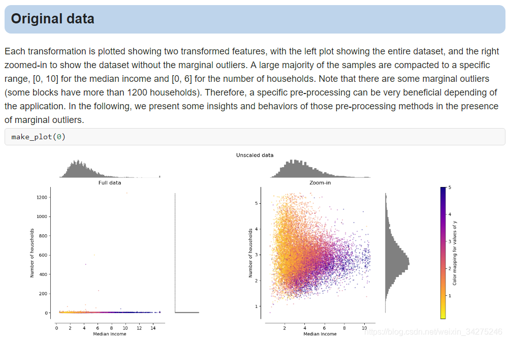
标签编码,字典向量化,特征散列
LabelEncoder和OneHotEncoder 在特征工程中的应用
对于性别,sex,一般的属性值是male和female。两个值。那么不靠谱的方法直接用0表示male,用1表示female 了。所以要用one-hot编码。
array([[0., 1.],
       [1., 0.],
       [0., 1.],
       [0., 1.],
       [1., 0.],
       [1., 0.]])
classes_:
Holds the label for each class
>>> from sklearn import preprocessing
>>> le = preprocessing.LabelEncoder()
>>> le.fit(["paris", "paris", "tokyo", "amsterdam"])
LabelEncoder()
>>> le.classes_
array(['amsterdam', 'paris', 'tokyo'], dtype='<U9')
>>> list(le.classes_)
['amsterdam', 'paris', 'tokyo']
from __future__ import print_function

import numpy as np

from sklearn.preprocessing import LabelEncoder, LabelBinarizer, OneHotEncoder
from sklearn.feature_extraction import DictVectorizer, FeatureHasher

# For reproducibility
np.random.seed(1000)


if __name__ == '__main__':
    Y = np.random.choice(('Male', 'Female'), size=(10))

    # Encode the labels
    print('Label encoding')
    le = LabelEncoder()
    yt = le.fit_transform(Y)
    print(yt)

    # Decode a dummy output
    print('Label decoding')
    output = [1, 0, 1, 1, 0, 0]
    decoded_output = [le.classes_[i] for i in output]
    print(decoded_output)

    # Binarize the labels
    print('Label binarization')
    lb = LabelBinarizer()
    yb = lb.fit_transform(Y)
    print(yb)

    # Decode the binarized labels
    print('Label decoding')
    lb.inverse_transform(yb)

    # Define some dictionary data
    data = [
        {'feature_1': 10, 'feature_2': 15},
        {'feature_1': -5, 'feature_3': 22},
        {'feature_3': -2, 'feature_4': 10}
    ]

    # Vectorize the dictionary data
    print('Dictionary data vectorization')
    dv = DictVectorizer()
    Y_dict = dv.fit_transform(data)
    print(Y_dict.todense())
    # toarray returns an ndarray; todense returns a matrix.

    print('Vocabulary:')
    print(dv.vocabulary_)

    # Feature hashing
    print('Feature hashing')
    fh = FeatureHasher()
    Y_hashed = fh.fit_transform(data)

    # Decode the features
    print('Feature decoding')
    print(Y_hashed.todense())

    # One-hot encoding
    data1 = [[0, 10, 0],
        	[1, 11, 1],
    	    [1, 8, 0],
  	        [0, 12, 0],
  	        [0, 15, 1]]

    # Encode data
    oh = OneHotEncoder()
    Y_oh = oh.fit_transform(data1)
    print(Y_oh.todense())
Label encoding
[0 0 0 1 0 1 1 0 0 1]

Label decoding
['Male', 'Female', 'Male', 'Male', 'Female', 'Female']

Label binarization
[[0]
 [0]
 [0]
 [1]
 [0]
 [1]
 [1]
 [0]
 [0]
 [1]]
Label decoding

Dictionary data vectorization
[[10. 15.  0.  0.]
 [-5.  0. 22.  0.]
 [ 0.  0. -2. 10.]]

Vocabulary:
{'feature_1': 0, 'feature_2': 1, 'feature_3': 2, 'feature_4': 3}

Feature hashing

Feature decoding
[[0. 0. 0. ... 0. 0. 0.]
 [0. 0. 0. ... 0. 0. 0.]
 [0. 0. 0. ... 0. 0. 0.]]


 [[1., 0., 0., 1., 0., 0., 0., 1., 0.]
  [0., 1., 0., 0., 1., 0., 0., 0., 1.]
  [0., 1., 1., 0., 0., 0., 0., 1., 0.]
  [1., 0., 0., 0., 0., 1., 0., 1., 0.]
  [1., 0., 0., 0., 0., 0., 1., 0., 1.]]
处理缺失数据
from __future__ import print_function

import numpy as np

from sklearn.preprocessing import Imputer

# For reproducibility
np.random.seed(1000)


if __name__ == '__main__':
    data = np.array([[1, np.nan, 2], [2, 3, np.nan], [-1, 4, 2]])
    print(data)

    # Imputer with mean-strategy
    print('Mean strategy')
    imp = Imputer(strategy='mean')
    print(imp.fit_transform(data))

    # Imputer with median-strategy
    print('Median strategy')
    imp = Imputer(strategy='median')
    print(imp.fit_transform(data))

    # Imputer with most-frequent-strategy
    print('Most-frequent strategy')
    imp = Imputer(strategy='most_frequent')
    print(imp.fit_transform(data))
[[ 1. nan  2.]
 [ 2.  3. nan]
 [-1.  4.  2.]]
Mean strategy
[[ 1.   3.5  2. ]
 [ 2.   3.   2. ]
 [-1.   4.   2. ]]
Median strategy
[[ 1.   3.5  2. ]
 [ 2.   3.   2. ]
 [-1.   4.   2. ]]
Most-frequent strategy
[[ 1.  3.  2.]
 [ 2.  3.  2.]
 [-1.  4.  2.]]
数据标准化
标准化(Standardization):对数据的分布的进行转换,使其符合某种分布(比如正态分布)的一种非线性特征变换。
method
2.1 Rescaling (min-max normalization)
2.2 Mean normalization
2.3 Standardization
2.4 Scaling to unit length
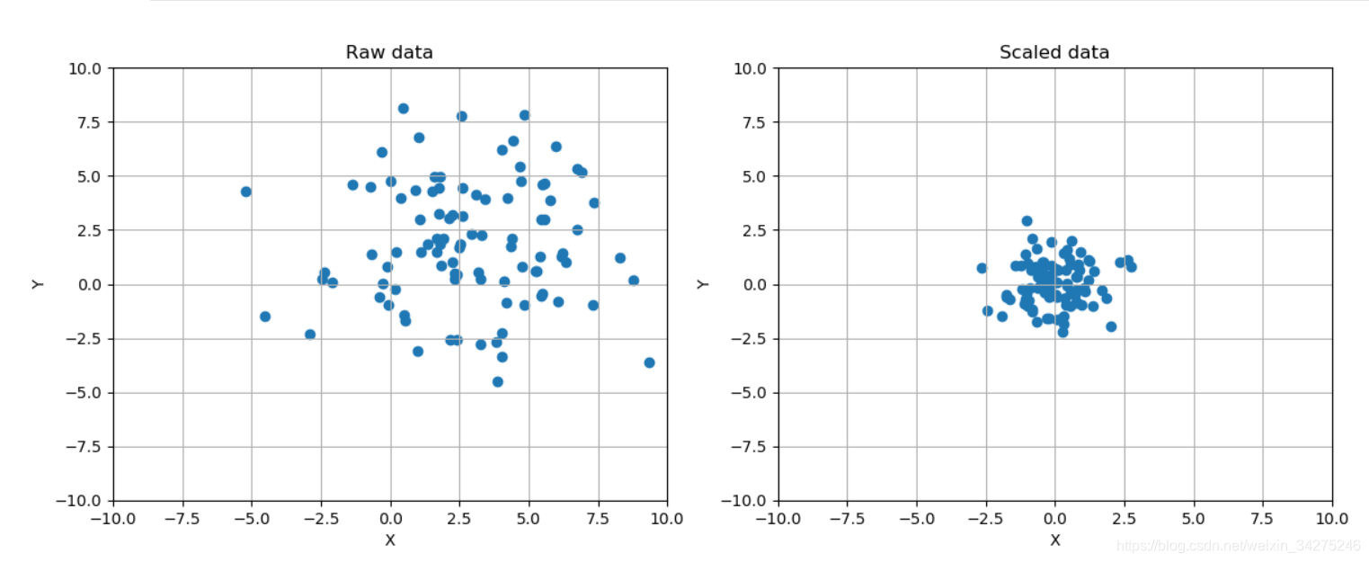
from __future__ import print_function

import numpy as np
import matplotlib.pyplot as plt

from sklearn.preprocessing import StandardScaler, RobustScaler

# For reproducibility
np.random.seed(1000)

if __name__ == '__main__':
    # Create a dummy dataset
    data = np.ndarray(shape=(100, 2))

    for i in range(100):
        data[i, 0] = 2.0 + np.random.normal(1.5, 3.0)
        data[i, 1] = 0.5 + np.random.normal(1.5, 3.0)

    # Show the original and the scaled dataset
    fig, ax = plt.subplots(1, 2, figsize=(14, 5))

    ax[0].scatter(data[:, 0], data[:, 1])
    ax[0].set_xlim([-10, 10])
    ax[0].set_ylim([-10, 10])
    ax[0].grid()
    ax[0].set_xlabel('X')
    ax[0].set_ylabel('Y')
    ax[0].set_title('Raw data')

    # Scale data
    ss = StandardScaler()
    scaled_data = ss.fit_transform(data)

    ax[1].scatter(scaled_data[:, 0], scaled_data[:, 1])
    ax[1].set_xlim([-10, 10])
    ax[1].set_ylim([-10, 10])
    ax[1].grid()
    ax[1].set_xlabel('X')
    ax[1].set_ylabel('Y')
    ax[1].set_title('Scaled data')

    plt.show()

    # Scale data using a Robust Scaler
    fig, ax = plt.subplots(2, 2, figsize=(8, 8))

    ax[0, 0].scatter(data[:, 0], data[:, 1])
    ax[0, 0].set_xlim([-10, 10])
    ax[0, 0].set_ylim([-10, 10])
    ax[0, 0].grid()
    ax[0, 0].set_xlabel('X')
    ax[0, 0].set_ylabel('Y')
    ax[0, 0].set_title('Raw data')

    rs = RobustScaler(quantile_range=(15, 85))
    scaled_data = rs.fit_transform(data)

    ax[0, 1].scatter(scaled_data[:, 0], scaled_data[:, 1])
    ax[0, 1].set_xlim([-10, 10])
    ax[0, 1].set_ylim([-10, 10])
    ax[0, 1].grid()
    ax[0, 1].set_xlabel('X')
    ax[0, 1].set_ylabel('Y')
    ax[0, 1].set_title('Scaled data (15% - 85%)')

    rs1 = RobustScaler(quantile_range=(25, 75))
    scaled_data1 = rs1.fit_transform(data)

    ax[1, 0].scatter(scaled_data1[:, 0], scaled_data1[:, 1])
    ax[1, 0].set_xlim([-10, 10])
    ax[1, 0].set_ylim([-10, 10])
    ax[1, 0].grid()
    ax[1, 0].set_xlabel('X')
    ax[1, 0].set_ylabel('Y')
    ax[1, 0].set_title('Scaled data (25% - 75%)')

    rs2 = RobustScaler(quantile_range=(30, 65))
    scaled_data2 = rs2.fit_transform(data)

    ax[1, 1].scatter(scaled_data2[:, 0], scaled_data2[:, 1])
    ax[1, 1].set_xlim([-10, 10])
    ax[1, 1].set_ylim([-10, 10])
    ax[1, 1].grid()
    ax[1, 1].set_xlabel('X')
    ax[1, 1].set_ylabel('Y')
    ax[1, 1].set_title('Scaled data (30% - 60%)')

    plt.show()
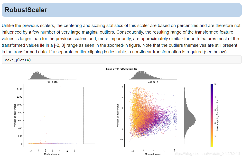
Compare the effect of different scalers on data with outliers
数据归一化
归一化:对数据的数值范围进行特定缩放,但不改变其数据分布的一种线性特征变换。
1.min-max 归一化:将数值范围缩放到(0,1),但没有改变数据分布;
2.z-score 归一化:将数值范围缩放到0附近, 但没有改变数据分布;
from __future__ import print_function

import numpy as np

from sklearn.preprocessing import Normalizer

# For reproducibility
np.random.seed(1000)

if __name__ == '__main__':
    # Create a dummy dataset
    data = np.array([1.0, 2.0, 8])
    print(data)

    # Max normalization
    n_max = Normalizer(norm='max')
    nm = n_max.fit_transform(data.reshape(1, -1))
    print(nm)

    # L1 normalization
    n_l1 = Normalizer(norm='l1')
    nl1 = n_l1.fit_transform(data.reshape(1, -1))
    print(nl1)

    # L2 normalization
    n_l2 = Normalizer(norm='l2')
    nl2 = n_l2.fit_transform(data.reshape(1, -1))
    print(nl2)
[1. 2. 8.]
[[0.125 0.25  1.   ]]
[[0.09090909 0.18181818 0.72727273]]
[[0.12038585 0.24077171 0.96308682]]
特征筛选
from __future__ import print_function

import numpy as np

from sklearn.datasets import load_boston, load_iris
from sklearn.feature_selection import SelectKBest, SelectPercentile, chi2, f_regression

# For reproducibility
np.random.seed(1000)

if __name__ == '__main__':
    # Load Boston data
    regr_data = load_boston()
    print('Boston data shape')
    print(regr_data.data.shape)

    # Select the best k features with regression test
    kb_regr = SelectKBest(f_regression)
    X_b = kb_regr.fit_transform(regr_data.data, regr_data.target)
    print('K-Best-filtered Boston dataset shape')
    print(X_b.shape)
    print('K-Best scores')
    print(kb_regr.scores_)

    # Load iris data
    class_data = load_iris()
    print('Iris dataset shape')
    print(class_data.data.shape)

    # Select the best k features using Chi^2 classification test
    perc_class = SelectPercentile(chi2, percentile=15)
    X_p = perc_class.fit_transform(class_data.data, class_data.target)
    print('Chi2-filtered Iris dataset shape')
    print(X_p.shape)
    print('Chi2 scores')
    print(perc_class.scores_)
Boston data shape
(506, 13)
K-Best-filtered Boston dataset shape
(506, 10)
K-Best scores
[ 88.15124178  75.2576423  153.95488314  15.97151242 112.59148028
 471.84673988  83.47745922  33.57957033  85.91427767 141.76135658
 175.10554288  63.05422911 601.61787111]
Iris dataset shape
(150, 4)
Chi2-filtered Iris dataset shape
(150, 1)
Chi2 scores
[ 10.81782088   3.59449902 116.16984746  67.24482759]
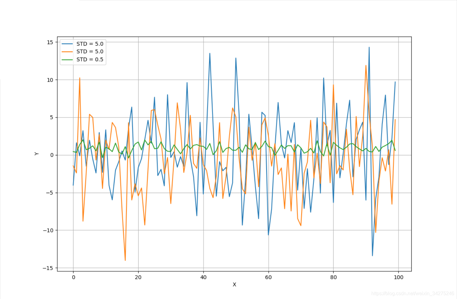
特征选择
from __future__ import print_function

import numpy as np
import matplotlib.pyplot as plt

from sklearn.feature_selection import VarianceThreshold

# For reproducibility
np.random.seed(1000)

if __name__ == '__main__':
    # Create a dummy dataset
    X = np.ndarray(shape=(100, 3))

    X[:, 0] = np.random.normal(0.0, 5.0, size=100)
    X[:, 1] = np.random.normal(0.5, 5.0, size=100)
    X[:, 2] = np.random.normal(1.0, 0.5, size=100)

    # Show the dataset
    fig, ax = plt.subplots(1, 1, figsize=(12, 8))
    ax.grid()
    ax.set_xlabel('X')
    ax.set_ylabel('Y')

    ax.plot(X[:, 0], label='STD = 5.0')
    ax.plot(X[:, 1], label='STD = 5.0')
    ax.plot(X[:, 2], label='STD = 0.5')

    plt.legend()
    plt.show()

    # Impose a variance threshold
    print('Samples before variance thresholding')
    print(X[0:3, :])

    vt = VarianceThreshold(threshold=1.5)
    X_t = vt.fit_transform(X)

    # After the filter has removed the componenents
    print('Samples after variance thresholding')
    print(X_t[0:3, :])
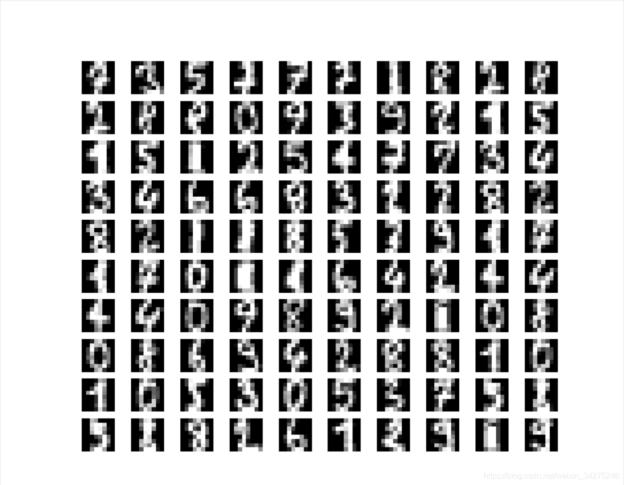
PCA
from __future__ import print_function
import numpy as np
import matplotlib.pyplot as plt
from sklearn.datasets import load_digits
from sklearn.decomposition import PCA
# For reproducibility
np.random.seed(1000)
if __name__ == '__main__':
# Load MNIST digits
digits = load_digits()
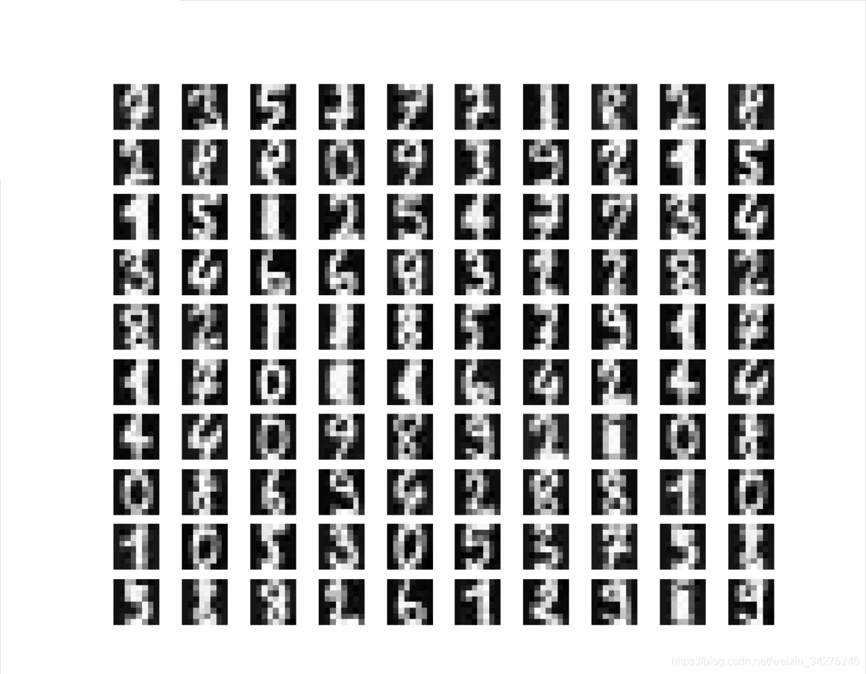
# Show some random digits
selection = np.random.randint(0, 1797, size=100)
fig, ax = plt.subplots(10, 10, figsize=(10, 10))
samples = [digits.data[x].reshape((8, 8)) for x in selection]
for i in range(10):
for j in range(10):
ax[i, j].set_axis_off()
ax[i, j].imshow(samples[(i * 8) + j], cmap='gray')
plt.show()
# Perform a PCA on the digits dataset
pca = PCA(n_components=36, whiten=True)
X_pca = pca.fit_transform(digits.data / 255)
print('Explained variance ratio')
print(pca.explained_variance_ratio_)
# Plot the explained variance ratio
fig, ax = plt.subplots(1, 2, figsize=(16, 6))
ax[0].set_xlabel('Component')
ax[0].set_ylabel('Variance ratio (%)')
ax[0].bar(np.arange(36), pca.explained_variance_ratio_ * 100.0)
ax[1].set_xlabel('Component')
ax[1].set_ylabel('Cumulative variance (%)')
ax[1].bar(np.arange(36), np.cumsum(pca.explained_variance_)[::-1])
plt.show()
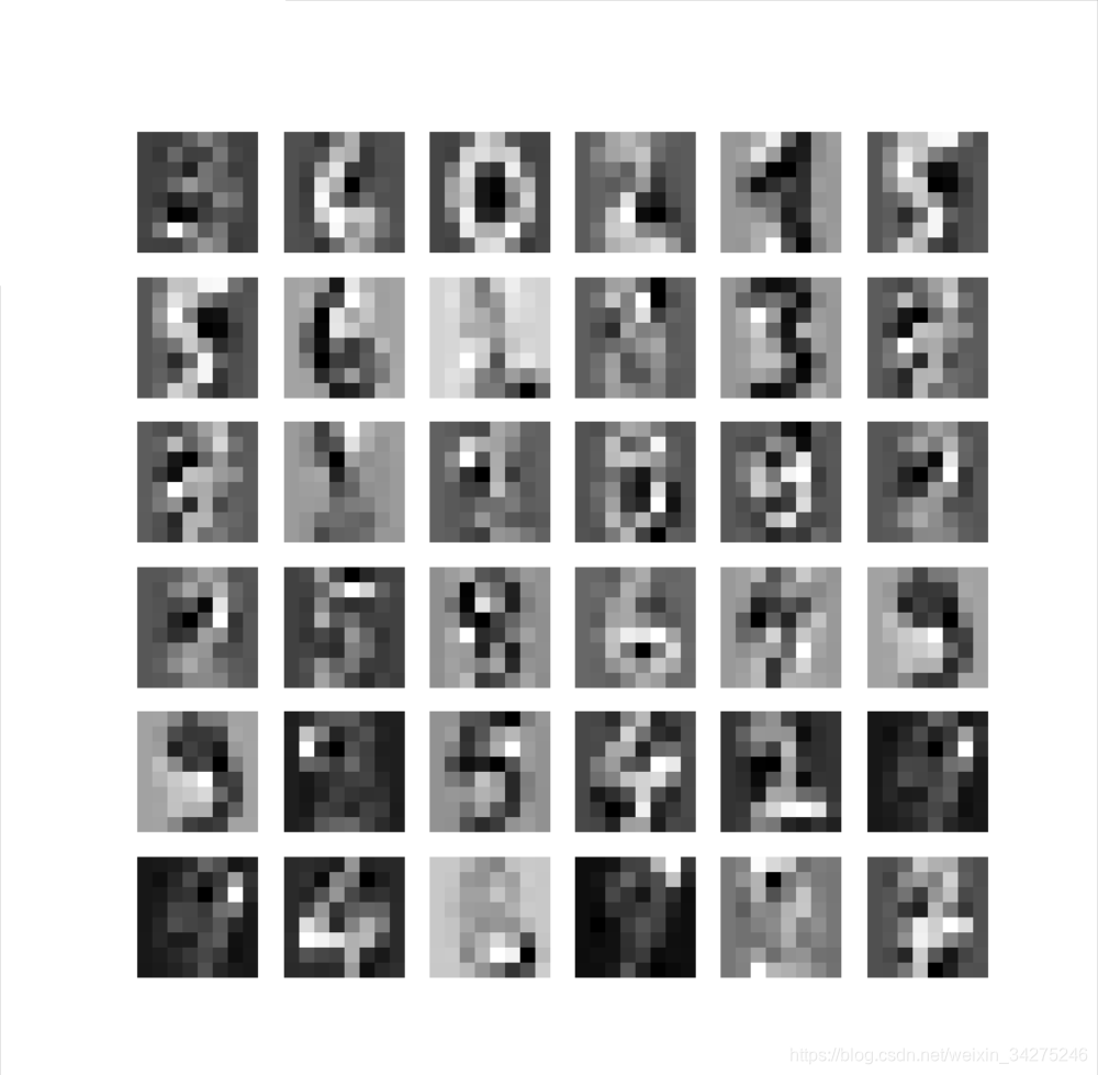
# Rebuild from PCA and show the result
fig, ax = plt.subplots(10, 10, figsize=(10, 10))
samples = [pca.inverse_transform(X_pca[x]).reshape((8, 8)) for x in selection]
for i in range(10):
for j in range(10):
ax[i, j].set_axis_off()
ax[i, j].imshow(samples[(i * 8) + j], cmap='gray')
plt.show()
Explained variance ratio
[0.14890594 0.13618771 0.11794594 0.08409979 0.05782415 0.0491691
 0.04315987 0.03661373 0.03353248 0.03078806 0.02372341 0.02272697
 0.01821863 0.01773855 0.01467101 0.01409716 0.01318589 0.01248138
 0.01017718 0.00905617 0.00889538 0.00797123 0.00767493 0.00722904
 0.00695889 0.00596081 0.00575615 0.00515158 0.0048954  0.00428887
 0.00373606 0.00353272 0.00336679 0.00328028 0.0030832  0.00293774]

DictionaryLearning
from __future__ import print_function

import numpy as np
import matplotlib.pyplot as plt

from sklearn.datasets import load_digits
from sklearn.decomposition import DictionaryLearning

# For reproducibility
np.random.seed(1000)

if __name__ == '__main__':
    # Load MNIST digits
    digits = load_digits()

    # Perform a dictionary learning (and atom extraction) from the MNIST dataset
    dl = DictionaryLearning(n_components=36, fit_algorithm='lars', transform_algorithm='lasso_lars')
    X_dict = dl.fit_transform(digits.data)

    # Show the atoms that have been extracted
    fig, ax = plt.subplots(6, 6, figsize=(8, 8))

    samples = [dl.components_[x].reshape((8, 8)) for x in range(34)]

    for i in range(6):
        for j in range(6):
            ax[i, j].set_axis_off()
            ax[i, j].imshow(samples[(i * 5) + j], cmap='gray')

    plt.show()
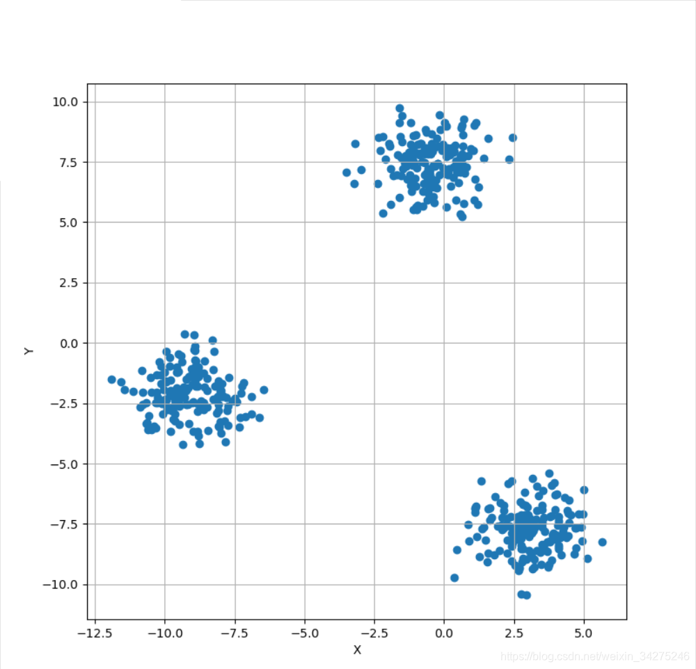
KPCA
from __future__ import print_function
import numpy as np
import matplotlib.pyplot as plt
from sklearn.datasets.samples_generator import make_blobs
from sklearn.decomposition import KernelPCA
# For reproducibility
np.random.seed(1000)
if __name__ == '__main__':
# Create a dummy dataset
Xb, Yb = make_blobs(n_samples=500, centers=3, n_features=3)
# Show the dataset
fig, ax = plt.subplots(1, 1, figsize=(8, 8))
ax.scatter(Xb[:, 0], Xb[:, 1])
ax.set_xlabel('X')
ax.set_ylabel('Y')
ax.grid()
plt.show()
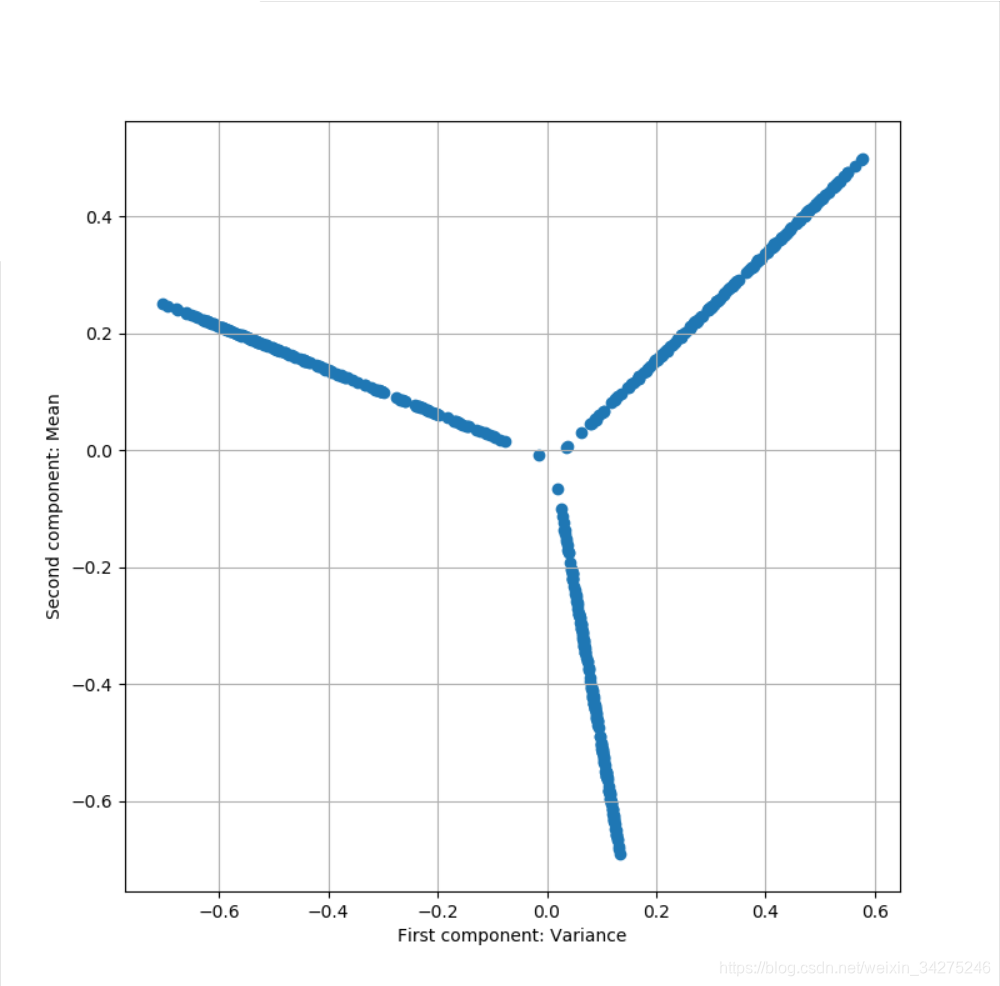
# Perform a kernel PCA (with radial basis function)
kpca = KernelPCA(n_components=2, kernel='rbf', fit_inverse_transform=True)
X_kpca = kpca.fit_transform(Xb)
# Plot the dataset after PCA
fig, ax = plt.subplots(1, 1, figsize=(8, 8))
ax.scatter(kpca.X_transformed_fit_[:, 0], kpca.X_transformed_fit_[:, 1])
ax.set_xlabel('First component: Variance')
ax.set_ylabel('Second component: Mean')
ax.grid()
plt.show()