特征选择
案例1:封装器法
常用实现方法:循序特征选择。
- 循序向前特征选择:Sequential Forward Selection,SFS
- 循序向后特征选择:Sequential Backword Selection,SBS
SFS
mlxtend
加载数据集
from mlxtend.feature_selection import SequentialFeatureSelector as SFS #SFS
from mlxtend.data import wine_data #dataset
from sklearn.neighbors import KNeighborsClassifier
from sklearn.model_selection import train_test_split
from sklearn.preprocessing import StandardScaler

X, y = wine_data()
X.shape

数据预处理
X_train, X_test, y_train, y_test= train_test_split(X, y, stratify=y, test_size=0.3, random_state=1)
std = StandardScaler()
X_train_std = std.fit_transform(X_train)
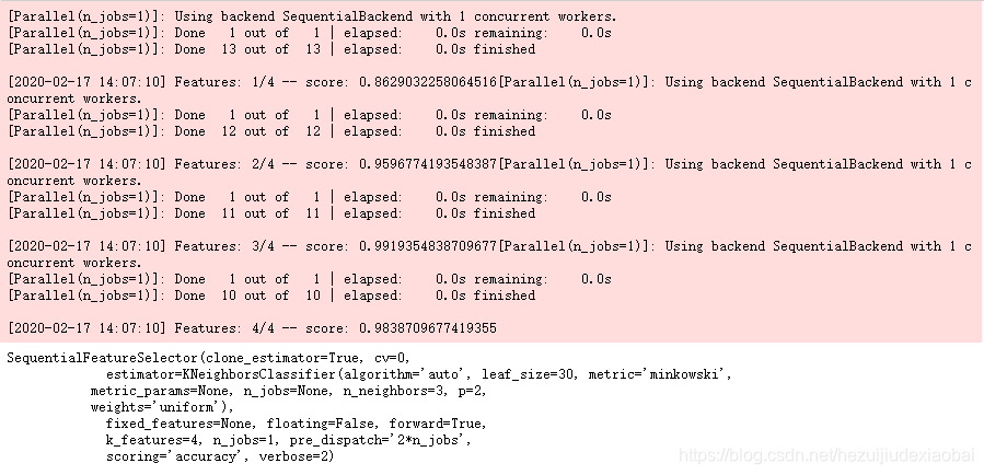
循序向前特征选择
knn = KNeighborsClassifier(n_neighbors=3)

sfs = SFS(estimator=knn, k_features=4, forward=True, floating=False, verbose=2, scoring='accuracy', cv=0)
sfs.fit(X_train_std, y_train)
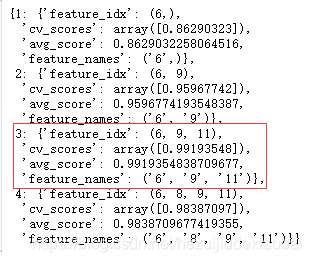
查看特征索引
Take a look at the selected feature indices at each step
sfs.subsets_
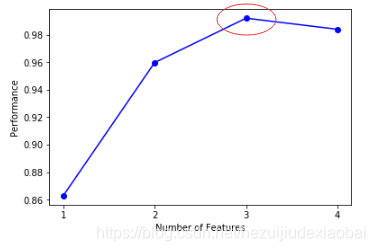
可视化#1
Plotting the results
%matplotlib inline
from mlxtend.plotting import plot_sequential_feature_selection as plot_sfs
fig = plot_sfs(sfs.get_metric_dict(), kind='std_err')
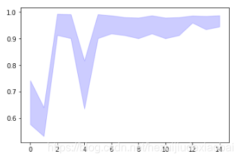
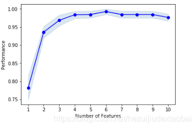
可视化#2
Selecting the “best” feature combination in a k-range
knn = KNeighborsClassifier(n_neighbors=3)
sfs2 = SFS(estimator=knn, k_features=(3, 10),
                   forward=True,
                   floating=True,
                   verbose=0,
                   scoring='accuracy',
                   cv=5)
sfs2.fit(X_train_std, y_train)
fig = plot_sfs(sfs2.get_metric_dict(), kind='std_err')
案例2:封装器之穷举特征选择
穷举特征选择(Exhaustive feature selection),即封装器中搜索算法是将所有特征组合都实现一遍,然后通过比较各种特征组合后的模型表现,从中选择出最佳的特征子集。
下载相关库
!pip install --upgrade pip

!pip install mlxtend
导入相关库
from mlxtend.feature_selection import ExhaustiveFeatureSelector as EFS
from sklearn.neighbors import KNeighborsClassifier
from sklearn.datasets import load_iris
加载数据集
iris = load_iris()
X = iris.data
y = iris.target
穷举特征选择
knn = KNeighborsClassifier(n_neighbors=3) # n_neighbors=3

efs = EFS(knn,
         min_features=1,
         max_features=4,
         scoring='accuracy',
         print_progress=True,
         cv=5)
efs = efs.fit(X, y)
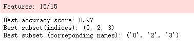
查看最佳特征子集
print('Best accuracy score: %.2f' % efs.best_score_)
print('Best subset(indices):', efs.best_idx_)
print('Best subset (correponding names):', efs.best_feature_names_)
更改特征名
feature_names = ('sepal length', 'sepal width', 'petal length', 'petal width')
efs = efs.fit(X, y, custom_feature_names=feature_names)
print('Best subset (corresponding names):', efs1.best_feature_names_)

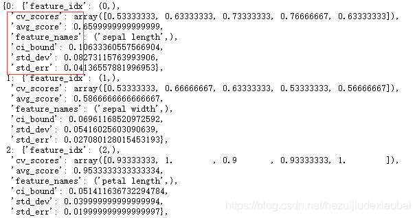
度量标准
efs.get_metric_dict()
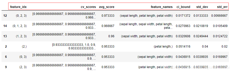
import pandas as pd

df = pd.DataFrame.from_dict(efs1.get_metric_dict()).T
df.sort_values('avg_score', inplace=True, ascending=False)
df
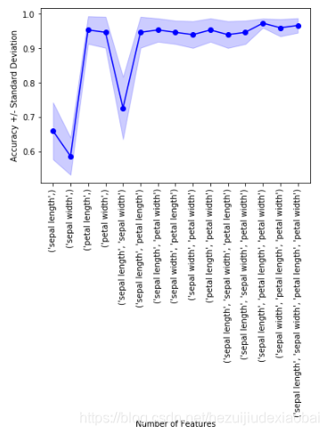
可视化
import matplotlib.pyplot as plt

# 平均值
metric_dict = efs.get_metric_dict()
k_feat = sorted(metric_dict.keys())
avg = [metric_dict[k]['avg_score'] for k in k_feat]

# 区域
fig = plt.figure()
upper, lower = [], []
for k in k_feat: #bound
    upper.append(metric_dict[k]['avg_score'] + metric_dict[k]['std_dev'])
    lower.append(metric_dict[k]['avg_score'] - metric_dict[k]['std_dev'])

plt.fill_between(k_feat, upper, lower, alpha=0.2, color='blue', lw=1)

# 折线图
plt.plot(k_feat, avg, color='blue', marker='o')

# x, y 轴标签
plt.ylabel('Accuracy +/- Standard Deviation')
plt.xlabel('Number of Features')
feature_min = len(metric_dict[k_feat[0]]['feature_idx'])
feature_max = len(metric_dict[k_feat[-1]]['feature_idx'])
plt.xticks(k_feat,
    [str(metric_dict[k]['feature_names']) for k in k_feat],
    rotation=90)
plt.show()
案例3:过滤器法
例1
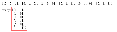
from sklearn.feature_selection import VarianceThreshold

X = [[0, 0, 1], [0, 1, 0], [1, 0, 0], [0, 1, 1], [0, 1, 0], [0, 1, 1]]
print(X)

sel = VarianceThreshold(threshold=(.8 * (1 - .8)))
sel.fit_transform(X)
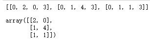
例2
X = [[0, 2, 0, 3], [0, 1, 4, 3], [0, 1, 1, 3]]
print(X)

seletor = VarianceThreshold()
seletor.fit_transform(X)
案例4:嵌入法
对系数排序——即特征权重,然后依据某个阈值选择部分特征。
在训练模型的同时,得到了特征权重,并完成特征选择。像这样,将特征选择过程与模型训练融为一体,在模型训练过程中自动进行了特征选择,被称为“嵌入法” (Embedded)特征选择。
例1
加载数据集
iris = load_iris()
X = iris.data
y = iris.target
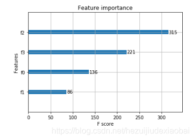
Xgboost特征重要性
from xgboost import XGBClassifier
model = XGBClassifier() # 分类
model.fit(X,y)
model.feature_importances_  # 特征重要性

可视化
%matplotlib inline
from xgboost import plot_importance
plot_importance(model)
例2
import matplotlib.pyplot as plt
import numpy as np
from sklearn.datasets import load_boston
from sklearn.feature_selection import SelectFromModel
from sklearn.linear_model import LassoCV
# Load the boston dataset.
X, y = load_boston(return_X_y=True)
# We use the base estimator LassoCV since the L1 norm promotes sparsity of features.
clf = LassoCV()
# Set a minimum threshold of 0.25
sfm = SelectFromModel(clf, threshold=0.25)
sfm.fit(X, y)
n_features = sfm.transform(X).shape[1]
# Reset the threshold till the number of features equals two.
# Note that the attribute can be set directly instead of repeatedly
# fitting the metatransformer.
while n_features > 2:
sfm.threshold += 0.1
X_transform = sfm.transform(X)
n_features = X_transform.shape[1]
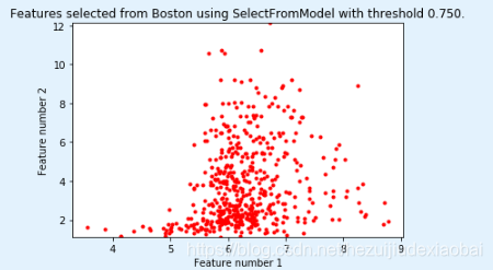
# Plot the selected two features from X.
plt.title(
"Features selected from Boston using SelectFromModel with " "threshold %0.3f." % sfm.threshold)
feature1 = X_transform[:, 0]
feature2 = X_transform[:, 1]
plt.plot(feature1, feature2, 'r.')
plt.xlabel("Feature number 1")
plt.ylabel("Feature number 2")
plt.ylim([np.min(feature2), np.max(feature2)])
plt.show()
例3
from sklearn.feature_selection import SelectFromModel
from sklearn.linear_model import LogisticRegression
X = [[ 0.87, -1.34, 0.31 ],
[-2.79, -0.02, -0.85 ],
[-1.34, -0.48, -2.55 ],
[ 1.92, 1.48, 0.65 ]]
y = [0, 1, 0, 1]
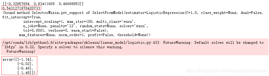
selector = SelectFromModel(estimator=LogisticRegression()).fit(X, y)
# The base estimator from which the transformer is built.
print(selector.estimator_.coef_)
# The threshold value used for feature selection.
print(selector.threshold_)
# Get a mask, or integer index, of the features selected
print(selector.get_support)
# Reduce X to the selected features.
selector.transform(X)
参考资料
pandas
help(pd.DataFrame.from_dict)
Construct DataFrame from dict of array-like or dicts.
Creates DataFrame object from dictionary by columns or by index allowing dtype sepecification.
help(pd.DataFrame.sort_values)
Sort by the values along either axis.
matplotlib
help(plt.fill_between)
Fill the area between two horizontal curves.
plt.fill_between(k_feat,
    upper,
    lower,
    alpha=0.2,
    color='blue',
    lw=1)