在上一篇博客中我们学习了逻辑回归(LogisticRegression)的理论。那么在这篇博客中,我们用代码展示一下,如何用梯度下降法获取逻辑回归的参数
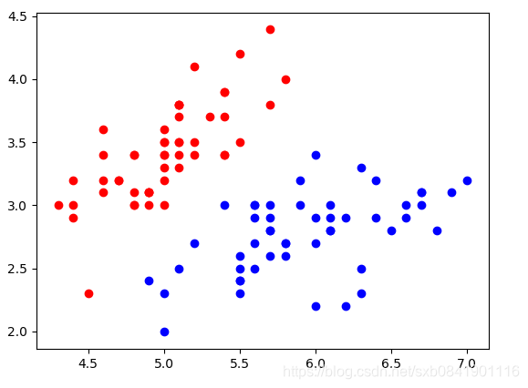
步骤1:我们加载sklearn中的鸢尾花数据进行测试,由于为了数据可视化,我们选择2种类型的鸢尾花,并且只选择2个特征。
    import numpy as np
    import matplotlib.pyplot as plt
    from sklearn import datasets

    X, y = datasets.load_iris(return_X_y=True)
    X = X[y < 2, :2]
    y = y[y < 2]
    plt.scatter(X[y == 0, 0], X[y == 0, 1], color="red")
    plt.scatter(X[y == 1, 0], X[y == 1, 1], color="blue")
    plt.show()
可视化一下:
步骤二: 我们编写自己的回归算法
# -*- encoding: utf-8 -*-
import numpy as np
from .metrics import accuracy_score

class LogisticRegression:

    def __init__(self):
        """初始化Logistic Regression模型"""
        self.coef_ = None
        self.intercept_ = None
        self._theta = None

    def _sigmoid(self, t):
        return 1. / (1. + np.exp(-t))

    def fit(self, X_train, y_train, eta=0.01, n_iters=1e4):
        """根据训练数据集X_train, y_train, 使用梯度下降法训练Logistic Regression模型"""
        assert X_train.shape[0] == y_train.shape[0], \
            "the size of X_train must be equal to the size of y_train"

        def J(theta, X_b, y):
            y_hat = self._sigmoid(X_b.dot(theta))
            try:
                return - np.sum(y*np.log(y_hat) + (1-y)*np.log(1-y_hat)) / len(y)
            except:
                return float('inf')

        def dJ(theta, X_b, y):
            return X_b.T.dot(self._sigmoid(X_b.dot(theta)) - y) / len(y)

        def gradient_descent(X_b, y, initial_theta, eta, n_iters=1e4, epsilon=1e-8):

            theta = initial_theta
            cur_iter = 0

            while cur_iter < n_iters:
                gradient = dJ(theta, X_b, y)
                last_theta = theta
                theta = theta - eta * gradient
                if (abs(J(theta, X_b, y) - J(last_theta, X_b, y)) < epsilon):
                    break

                cur_iter += 1

            return theta

        X_b = np.hstack([np.ones((len(X_train), 1)), X_train])
        initial_theta = np.zeros(X_b.shape[1])
        self._theta = gradient_descent(X_b, y_train, initial_theta, eta, n_iters)

        self.intercept_ = self._theta[0]
        self.coef_ = self._theta[1:]

        return self

    def predict_proba(self, X_predict):
        """给定待预测数据集X_predict,返回表示X_predict的结果概率向量"""
        assert self.intercept_ is not None and self.coef_ is not None, \
            "must fit before predict!"
        assert X_predict.shape[1] == len(self.coef_), \
            "the feature number of X_predict must be equal to X_train"

        X_b = np.hstack([np.ones((len(X_predict), 1)), X_predict])
        return self._sigmoid(X_b.dot(self._theta))

    def predict(self, X_predict):
        """给定待预测数据集X_predict,返回表示X_predict的结果向量"""
        assert self.intercept_ is not None and self.coef_ is not None, \
            "must fit before predict!"
        assert X_predict.shape[1] == len(self.coef_), \
            "the feature number of X_predict must be equal to X_train"

        proba = self.predict_proba(X_predict)
        return np.array(proba >= 0.5, dtype='int')

    def score(self, X_test, y_test):
        """根据测试数据集 X_test 和 y_test 确定当前模型的准确度"""

        y_predict = self.predict(X_test)
        return accuracy_score(y_test, y_predict)

    def __repr__(self):
        return "LogisticRegression()"
步骤三、进行测试
    from logisticregression import LogisticRegression
    iris = load_iris()
    X = iris.data
    y = iris.target
    X = X[y < 2, :2]
    y = y[y < 2]
    log_reg = LogisticRegression()
    X_train, X_test, y_train, y_test = train_test_split(X, y, random_state=666)
    log_reg.fit(X_train, y_train)
    print log_reg.theta_
    print log_reg.predict_probality(X_test)
    print log_reg.predict(X_test)
    print log_reg.scores(X_test, y_test)
运行结果:
参数: 第1个表示截距, 第2,3表示参数: [ 0. 2.93348784 -5.10537984]
预测出来的概率:
[0.92944114 0.98777304 0.15845401 0.18960373 0.03911344 0.02054764
0.05175747 0.99672293 0.9787036 0.7523886 0.04525759 0.003409
0.28048662 0.03911344 0.83661026 0.81299828 0.83506118 0.34328248
0.06419014 0.22523806 0.02384776 0.17983628 0.9787036 0.98804275
0.08845609]把概率进行映射出来的结果:
[1 1 0 0 0 0 0 1 1 1 0 0 0 0 1 1 1 0 0 0 0 0 1 1 0]准确率为:
1这个主要是由于数据比较少,并且我们只取了2个特征,不复杂。所以评分高。
总结:
1、在代码实现过程中,梯度下降方法中初始化init_theta错了,后来参考了一下老师的代码,重新改正过来了。
init_theta = np.zeros(X_b.shape[1]) 这里面X_b已经增加了一列。 这个要注意。 要是你在西安,感兴趣一起学习AIOPS,欢迎加入QQ群 860794445