R语言中基本图形的绘制

条形图

简单的垂直条形图和水平条形图

函数barplot()

> library(vcd)
载入需要的程辑包：grid
> counts <- table(Arthritis$Improved)
> counts

  None   Some Marked 
    42     14     28 
> barplot(counts,main = "Simple Bar Plot",xlab = "Improved",ylab = "Frequency") 
> barplot(counts,main = "Horizontal Bar Plot",xlab = "Improved",ylab = "Frequency",horiz = TRUE)

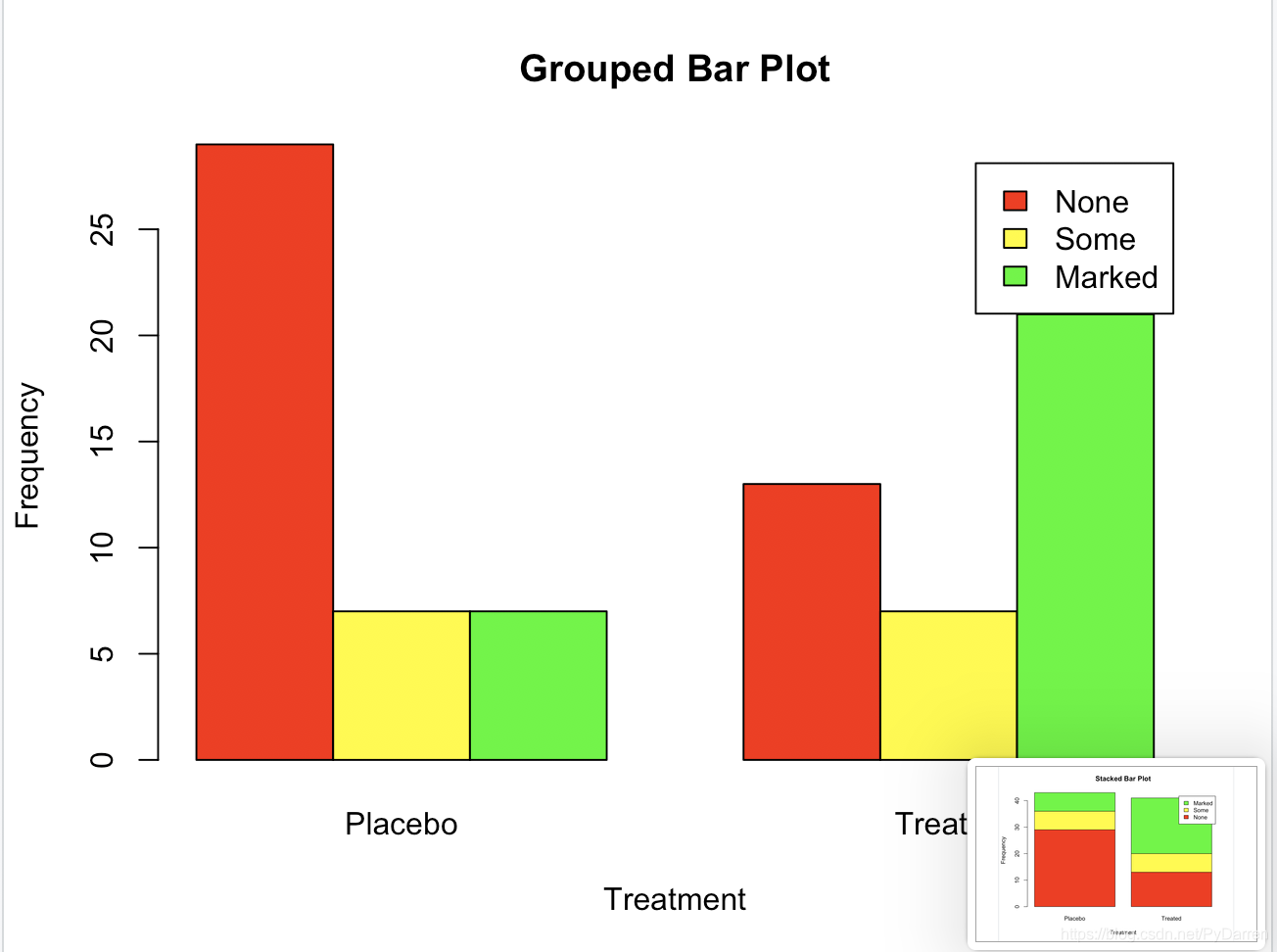
堆砌条形图和分组条形图

若beside=FALSE（默认值）则每一列都将生成图中的一个条形，各列中的值将给出堆砌的“子条”的高度。若base=TRUE则矩阵中的每一列都表示一个分组，各列中的值将并列而不是堆砌。

library(vcd)

counts <- table(Arthritis$Improved,Arthritis$Treatment)
counts

#堆砌条形图
barplot(counts,
        main = "Stacked Bar Plot",
        xlab = "Treatment",ylab = "Frequency",
        col = c("red","yellow","green"),
        legend = rownames(counts))

#分组条形图
barplot(counts,
        main = "Grouped Bar Plot",
        xlab = "Treatment", ylab = "Frequency",
        col = c("red","yellow","green"),
        legend = rownames(counts),
        beside = TRUE)

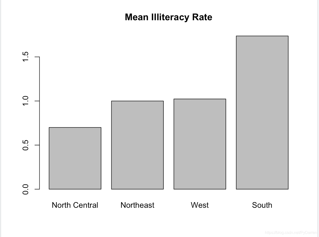
均值条形图

条形图不一定要基于计数数据或频率数据。可以使用数据整合函数并将结果传递给barplot()函数，来创建表示均值、中位数、标准差等的条形图。

#美国各地区平均文盲率排序的条形图
states <- data.frame(state.region,state.x77)
means <- aggregate(states$Illiteracy,by=list(state.region),FUN=mean)

means <- means[order(means$x),]
means

barplot(means$x,names.arg = means$Group.1)
title("Mean Illiteracy Rate")

条形图的微调

随着条形图条数的增多，条形的标签可能会开始重叠，可以使用cex.names来减小字号，将其指定为小于1的值可以缩小标签的大小。可选的参数names.arg允许你指定一个字符向量作为条形的标签名，同样可以使用图形参数辅助调整文本间隔。

####为条形图搭配标签

#增加y边界的大小
par(mar=c(5,8,4,2))
#旋转条形的标签
par(las=2)

counts <- table(Arthritis$Improved)

barplot(counts,
        main = "Treatment Outcome",
        horiz = TRUE,
        cex.names = 0.8,  #缩小字体大小，让标签更合适
        names.arg = c("No Improvement","Some Improvement",    #修改标签文本
                      "Marked Improvement"))

棘状图

棘状图对堆砌条形图进行了重缩放，这样让每个条形的高度为1，每一段的高度即表示比例。可由vcd包中的函数spine（）绘制。

library(vcd)

attach(Arthritis)
counts <- table(Treatment,Improved)
spine(counts,main = "Spinogram Example")
detach(Arthritis)

饼图

饼图在商业世界中应用广泛，但是在学术领域往往被否定，这是因为相对于面积，人们对长度的判断更精确。通过pie(x,labels）函数来创建。

par(mfrow=c(2,2))     #将四幅图组合为一幅

slices <- c(10,12,4,16,8)
lbls <- c("US","UK","Australia","Germany","France")
pie(slices,labels = lbls,
    main = "Simple Pie Chart")

pct <- round(slices / sum(slices) * 100)    #为饼图添加比例数值
lbls2 <- paste(lbls," ",pct,"%",sep = "")
pie(slices,labels = lbls2, col = rainbow(length(lbls2)),
    main = "Pie Chart with Percentages")

library(plotrix)
pie3D(slices,labels = lbls,explode = 0.1,
      main="3D Pie Chart")

my_table <- table(state.region)
lbls3 <- paste(names(my_table),"\n",my_table,sep = "")
pie(my_table,labels = lbls3,
    main = "Pie Chart from a Table\n (with sample sizes)")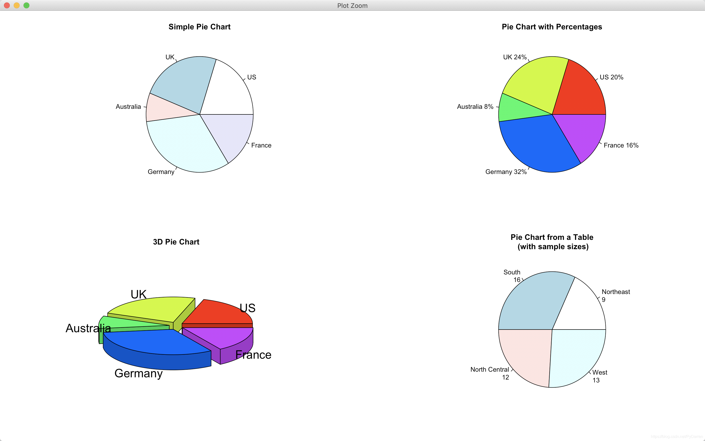

扇形图

通过plotrix包中的fan.plot()函数实现的。

library(plotrix)

slices <- c(10,12,4,16,8)
lbls <- c("US","UK","Australia","Germany","France")
fan.plot(slices,labels = lbls, main = "Fan Plot")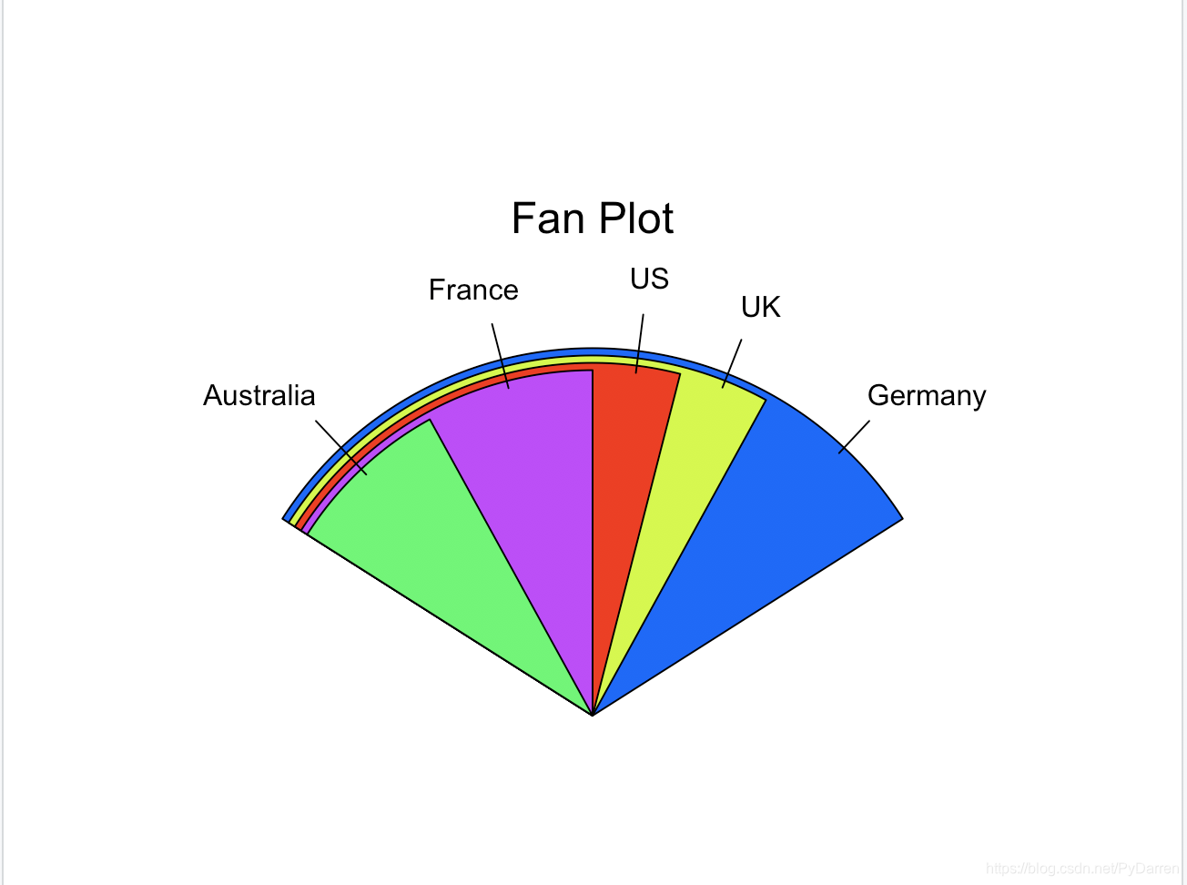

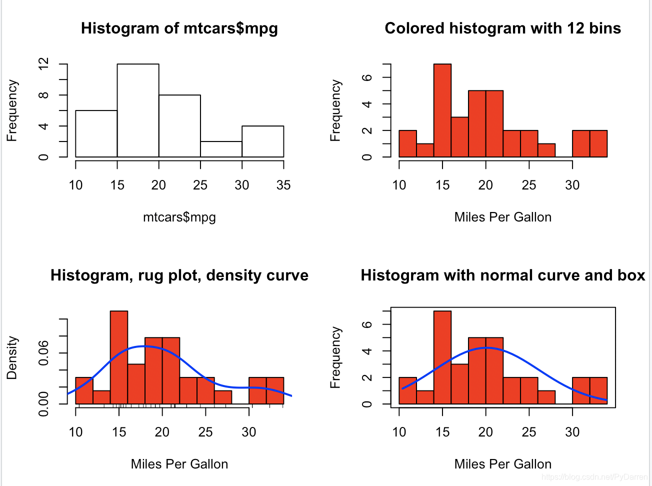
直方图

通过函数hist()创立。其中参数freq=FALSE表示根据概率密度而不是频数绘制图形，参数breaks用于控制组的数量。

par(mfrow = c(2,2))

#简单的直方图
hist(mtcars$mpg)

#指定组数和颜色
hist(mtcars$mpg,
     breaks = 12,
     col = "red",
     xlab = "Miles Per Gallon",
     main = "Colored histogram with 12 bins")

#添加轴须图
hist(mtcars$mpg,
     freq = FALSE,
     breaks = 12,
     col = "red",
     xlab = "Miles Per Gallon",
     main = "Histogram, rug plot, density curve")
rug(jitter(mtcars$mpg))
lines(density(mtcars$mpg), col = "blue", lwd = 2)

#添加正态密度曲线和外框
x <- mtcars$mpg
h <- hist(x,
          breaks = 12,
          col = "red",
          xlab = "Miles Per Gallon",
          main = "Histogram with normal curve and box")
xfit <- seq(min(x), max(x), length = 40)
yfit <- dnorm(xfit, mean = mean(x), sd = sd(x))
yfit <- yfit * diff(h$mids[1:2]) *length(x)
lines(xfit, yfit, col = "blue", lwd = 2)
box()