图像跟踪与识别-KCF+DSST算法简单融合

一：KCF高速跟踪详解

本文的跟踪方法效果甚好，速度奇高，思想和实现均十分简洁。其中利用循环矩阵进行快速计算的方法尤其值得学习。另外，作者在主页上十分慷慨地给出了各种语言的实现代码。
本文详细推导论文中的一系列步骤，包括论文中未能阐明的部分。请务必先参看这篇简介循环矩阵性质的博客。

思想

一般化的跟踪问题可以分解成如下几步：
1. 在It帧中，在当前位置pt附近采样，训练一个回归器。这个回归器能计算一个小窗口采样的响应。
2. 在It+1帧中，在前一帧位置pt附近采样，用前述回归器判断每个采样的响应。
3. 响应最强的采样作为本帧位置pt+1。

循环矩阵表示图像块

在图像中，循环位移操作可以用来近似采样窗口的位移。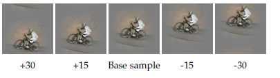
这里写图片描述
训练时，围绕着当前位置进行的一系列位移采样可以用二维分块循环矩阵X表示，第ij块表示原始图像下移i行右移j列的结果。类似地，测试时，前一帧结果附近的一系列位移采样也可以用X表示。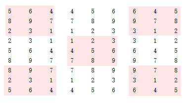

这样的X可以利用傅里叶变换快速完成许多线性运算。

线性回归训练提速

此部分频繁用到了循环矩阵的各类性质，请参看这篇博客。
线性回归的最小二乘方法解为：

w = (X H X + λ I) - 1 X H y

根据循环矩阵乘法性质，XHX的特征值为x^⊙x^∗。I本身就是一个循环矩阵，其生成向量为[1,0,0...0]，这个生成向量的傅里叶变换为全1向量，记为δ。

w = (F d i a g (x^⊙ x^*) F H + λ F d i a g (δ) F H) - 1 X H y

= (F d i a g (x^⊙ x^* + λ δ) F H) - 1 X H y

根据循环矩阵求逆性质，可以把矩阵求逆转换为特征值求逆。

w = F \cdot d i a g (1 x ^ ⊙ x ^ * + λ δ) \cdot F H X H y

w = F \cdot d i a g (1 x ^ ⊙ x ^ * + λ δ) \cdot F H \cdot F d i a g (x^*) F H \cdot y

利用F的酉矩阵性质消元：

w = F \cdot d i a g (x ^ * x ^ ⊙ x ^ * + λ δ) \cdot F H \cdot y

分号表示用1进行对位相除。
反用对角化性质：Fdiag(y)FH=C(F−1(y))，上式的前三项还是一个循环矩阵。

w = C (F - 1 (x ^ * x ^ ⊙ x ^ * + λ δ)) \cdot y

利用循环矩阵卷积性质F(C(x)⋅y)=x^∗⊙y^：

F (w) = (x ^ * x ^ ⊙ x ^ * + λ δ) * ⊙ F (y)

由于

x^⊙x^∗ 的每个元素都是实数，所以共轭不变：

F (w) = x ^ x ^ ⊙ x ^ * + λ δ ⊙ F (y) = x ^ ⊙ y ^ x ^ ⊙ x ^ * + λ δ

论文中，最后这一步推导的分子部分写成x^∗⊙y^，是错误的。但代码中没有涉及。

线性回归系数ω可以通过向量的傅里叶变换和对位乘法计算得到。

核回归训练提速

不熟悉核方法的同学可以参看这篇博客的简单说明。核回归方法的回归式为：

f (z) = α T κ (z)

其中

κ(z) 表示测试样本

z 和所有训练样本的核函数。参数有闭式解：

α = (K + λ I) - 1 y

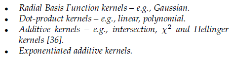
K为所有训练样本的核相关矩阵：Kij=κ(xi,xj)。如果核函数选择得当，使得x内部元素顺序更换不影响核函数取值，则可以保证K也是循环矩阵。以下核都满足这样的条件：
这里写图片描述

设核相关矩阵的生成向量是k。推导和之前线性回归的套路非常类似：

α = (F d i a g (k^) F H + F d i a g (λ δ) F H) - 1 y = (F d i a g (k^+ λ δ) F H) - 1 y

= F d i a g (1 k ^ + λ δ) F H y = C (F - 1 (1 k ^ + λ δ)) y

利用循环矩阵卷积性质F(C(x)⋅y)=x^∗⊙y^：

α^= (1 k ^ + λ δ) * ⊙ y^

这里

k 是核相关矩阵的第一行，表示原始生成向量

x0 和移位了

i 的向量

xi 的核函数。考察其处于对称位置上的两个元素：

k i = κ (x 0, x i), k N - i = κ (x 0, x N - i)

两者都是同一个向量和自身位移结果进行运算。因为所有涉及到的核函数都只和位移的绝对值有关，所以ki=kN−i，即k是对称向量。

举例：x0=[1,2,3,4]，x1=[4,1,2,3]，x3=[2,3,4,1]。使用多项式核κ(x,y)=xTy，容易验证κ(x0,x1)=κ(x0,x3)。

对称向量的傅里叶变换为实数，有：

α^= (1 k ^ + λ δ) ⊙ y^= y ^ k ^ + λ δ

论文中，利用k的对称性消除共轭的步骤没有提及。

线性回归系数α可以通过向量的傅里叶变换和对位乘法计算得到。

核回归检测提速

所有待检测样本和所有训练样本的核相关矩阵为K，每一列对应一个待测样本。可以一次计算所有样本的响应（N×1向量）：

y' = K T α

利用循环矩阵的转置性质性质，C(k)的特征值为k^∗：

y' = C (k) T \cdot α = C (k^*) \cdot α = k * * α

利用循环矩阵的卷积性质：

y' = (k *) * α = k * α

两边傅里叶变换：

y'^= k^⊙ α^

论文中，利用转置消除共轭的步骤没有提及。

所有侯选块的检测响应可以通过向量的傅里叶变换和对位乘法计算得到。

核相关矩阵计算提速

无论训练还是检测，都需要计算核相关矩阵K的生成向量k。除了直接计算每一个核函数，在某些特定的核函数下可以进一步加速。

多项式核

κ (x, y) = f (x T y)

其中f为多项式函数。写成矩阵形式：

K = f (X T Y)

f在矩阵的每个元素上单独进行。根据循环矩阵性质，XTY也是一个循环矩阵，其生成向量为F−1(y^⊙x^∗)。所以核相关矩阵的生成向量为：

k = f (F - 1 (y^⊙ x^*))

RBF核

κ (x, y) = f (| | x - y | | 2)

其中

f 是线性函数。简单展开：

κ (x, y) = f (| | x - y | | 2) = f (| | x | | 2 + | | y | | 2 + 2 x T y)

由于

X 中的所有

x 都通过循环移位获得，故

||x||2 对于所有

x 是常数，同理

||y||2 也是。所以核相关矩阵的生成向量为：

k = f (| | x | | 2 + | | y | | 2 + F - 1 (y^⊙ x^*))

其他核

有一些核函数，虽然能保证K是循环矩阵，但无法直接拆解出其特征值，快速得到生成向量。比如Hellinger核：∑ixiyi−−−√，Intersection核：∑imin(xi,yi)。

多通道

在多通道情况下（例如使用了HOG特征），生成向量x变成M×L，其中M是样本像素数，L是特征维度。在上述所有计算中，需要更改的只有向量的内积：

x T y = \sum l (x l) T y l

注：非常感谢GX1415926535和大家的帮助，发现原文一处错误。(21)式中不应有转置，应为：

f(z)=Kzα

二：DSST
简介(Accurate Scale Estimation for Robust Visual Tracking)

DSST(Discriminative Scale Space Tracking)在2014年VOT上夺得了第一名，算法简洁，性能优异，并且我上一篇所述的KCF夺得了第三名，两者都是基于滤波器的算法，这一年是CF义军突起的一年，值得研究这些相近的优秀算法。这篇算法是基于MOSSE的改进，突出内容是加入了尺度变换，下面开始逐一讲解算法内容。

相关滤波器

　　首先讲一下MOSSE提出的相关滤波器，从目标中提取一系列的图像patches,记为
f1,f2,...ft作为训练样本，其对应的滤波器响应值为一个个高斯函数 g1,g2,...gt,而目的就是找到满足最小均方差(Minimum Output Sum of Squared Error)的最优滤波器：

ε=∑j=1t||ht∗fj−gj||2=1MN||HtFj−Gj||2(1)

其中第二个等号根据Parseval定理导出，等式左侧是空域的方程式，右侧是频域的方程式，正正是这个等式，使得我们将问题求解变换到频域里求解， ε 的最小值在频域里的解如下：

Ht=∑tj=1GjFj∑tj=1FjFj(2)

一般而言， gj 可以是任意形状的输出，这里的输出 gj 是高斯型的函数，峰值位于中心处。这个方法的技巧或者目的在于：一是运算简洁，基本都是矩阵运算；二是引入快速傅里叶(FFT)大大加快运算效率。这即是相关滤波器被应用在Tracking并获得较好效果的原因，满足了对速度的一大需求。
在得到上述相关滤波器后，对于新的一帧中的候选输入样本z,求相关得分y：

y=−1(HtZ)(3)

y取最大响应值时对应的位置z为新的目标位置。
算法思想

　　算法设计了两个一致的相关滤波器，分别实现目标的跟踪和尺度变换，定义为位置滤波器(translation filter)和尺度滤波器(scale filter),前者进行当前帧目标的定位，后者进行当前帧目标尺度的估计。两个滤波器是相对独立的，从而可以选择不同的特征种类和特征计算方式来训练和测试。文中指出该算法亮点是尺度估计的方法可以移植到任意算法中去。

算法流程：如上图所示，通过左侧的图像patch目标提取的特征F和右侧的高斯型函数G，应用式(2)得到一个相关滤波器H。然后在下一帧将测试的图像patches提取特征Z作为输入，与相关滤波器H按照式(3)进行运算，得到响应值y最大的候选目标，所以算法很简洁。
该算法将输入信号 f(图像中的某一个patch)设计为d维特征向量(可选gray,hog)，通过建立最小化代价函数构造最优相关滤波器 h,如下：
$ε = | | \sum l = 1 d h l * f l - g | | 2 + λ \sum l = 1 d | | h l | | 2 (4)$
其中， l表示特征的某一维度， λ是正则项系数，作用是消除 f频谱中的零频分量的影响，避免上式解的分子为零，如下：
$H l = G ⎯ ⎯ ⎯ F l \sum d k = 1 F k ⎯ ⎯ ⎯ ⎯ F k + λ = A l t B t (5)$
由于patch中的每个像素点需要求解 dx d维的线性方程，计算非常耗时，为了得到鲁棒的近似结果，对上式中分子 Alt和分母 Bt分别进行更新:
$A l t = (1 - η) A l t - 1 + η G t ⎯ ⎯ ⎯ ⎯ F l t$
$B t = (1 - η) B t - 1 + η \sum k = 1 d F k t ⎯ ⎯ ⎯ ⎯ F l t (6)$
其中， η为学习率。
在新的一帧中，目标位置可以通过求解最大相关滤波器响应值得到：
$y =  - 1 ⎧ ⎩ ⎨ ⎪ ⎪ \sum d l = 1 A l ⎯ ⎯ ⎯ ⎯ Z l B + λ ⎫ ⎭ ⎬ ⎪ ⎪ (7)$

快速尺度空间跟踪

　　本算法的亮点就是提出的基于一维独立的相关滤波器的尺度搜索和目标估计方法。具体操作方法是：在新的一帧中，先利用2维的位置相关滤波器来确定目标的新候选位置，再利用1维的尺度相关滤波器以当前中心位置为中心点，获取不同尺度的候选patch，从而找到最匹配的尺度。尺寸选择原则是：

anP×anR,n∈{[−S−12],...[S−12]}

其中， P,R 分别为目标在前一帧的宽高， a=1.02 为尺度因子， S=33 为尺度的数量。上述尺度不是线性关系，而是由精到粗(从内到外的方向)的检测过程。
算法流程

　　论文中的流程图已经详细写的挺详细了，为了保持内容完整性再赘述一遍：
Input:
输入图像patch It
上一帧的位置Pt−1和尺度St−1
位置模型Atranst−1、Btanst−1和尺度模型Ascalet−1、Bscalet−1
Output:
估计的目标位置Pt和尺度St
更新位置Atranst、Btranst和尺度模型Ascalet、Bscalet

其中,
位置评估：
1.参照模板在前一帧的位置，在当前帧中按照前一帧目标尺度的2倍大小提取一个样本Ztrans
2.利用Ztrans和Atranst−1、Btanst−1，根据公式(7)计算ytrans
3.计算max(ytrans)，得到目标新的位置Pt
尺度评估：
4.以目标当前新位置为中心，提取33种不同尺度的样本Ztrans
5.利用Ztrans和Atranst−1、Btanst−1计算出yscale
6.计算max(yscale)，得到目标准确的尺度St

模型更新：
7.提取样本ftrans和fscale
8.更新位置模型Atranst和Btranst
9.更新尺度模型Ascalet和Bscalet

下面给出两个不同相关滤波器的关键代码：
训练部分：
    %提取特征训练样本输入X
    %样本中每个像素点计算28维融合特征(1维原始灰度+27维fhog)
    %乘以二维hann后作为输入X
    %提取特征用于位置相关滤波器
    xl = get_translation_sample(im, pos, sz, currentScaleFactor, cos_window);

    %获取分子A=GF;分母B=F*F;此时没有lambda
    xlf = fft2(xl);
    new_hf_num = bsxfun(@times, yf, conj(xlf));
    new_hf_den = sum(xlf .* conj(xlf), 3);

    %把每个样本resize成固定大小，分别提取31维fhog特征，每个样本的所有fhog再
    %串联成一个特征向量构成33层金字塔特征，乘以一维hann窗后作为输入X
    % 提取特征用于尺度相关滤波器
    xs = get_scale_sample(im, pos, base_target_sz, currentScaleFactor * scaleFactors, scale_window, scale_model_sz);

    %同样的获取分子A=GF;分母B=F*F;此时没有lambda
    xsf = fft(xs,[],2);
    new_sf_num = bsxfun(@times, ysf, conj(xsf));
    new_sf_den = sum(xsf .* conj(xsf), 1);
检测部分：
         %提取特征测试输入F
         %样本中每个像素点计算28维融合特征(1维原始灰度+27维fhog)
         %乘以二维hann后作为输入F
         %用于位置相关滤波器
         xt = get_translation_sample(im, pos, sz, currentScaleFactor, cos_window);

        %计算响应值y=F-1{(A*Z)/(B+lambda)}
        xtf = fft2(xt);
        response = real(ifft2(sum(hf_num .* xtf, 3) ./ (hf_den + lambda)));

        %找到max(y)得到目标新位置
        [row, col] = find(response == max(response(:)), 1);

        % 更新目标位置
        pos = pos + round((-sz/2 + [row, col]) * currentScaleFactor);

        %把每个样本resize成固定大小，分别提取31维fhog特征，每个样本的所有fhog再
        %串联成一个特征向量构成33层金字塔特征，乘以一维hann窗后作为输入F
        % 用于尺度相关滤波器
        xs = get_scale_sample(im, pos, base_target_sz, currentScaleFactor * scaleFactors, scale_window, scale_model_sz);

        %得到尺度变换的响应最大值y=F-1{(A*Z)/(B+lambda)}
        xsf = fft(xs,[],2);
        scale_response = real(ifft(sum(sf_num .* xsf, 1) ./ (sf_den + lambda)));

        %找到max(y)得到当前的尺度
        recovered_scale = find(scale_response == max(scale_response(:)), 1);

        % 更新当前尺度
        currentScaleFactor = currentScaleFactor * scaleFactors(recovered_scale);
        if currentScaleFactor < min_scale_factor
            currentScaleFactor = min_scale_factor;
        elseif currentScaleFactor > max_scale_factor
            currentScaleFactor = max_scale_factor;
        end
总结

　　DSST算法是一个非常典型且高效的基于相关滤波器的目标跟踪算法，非常值得学习和借鉴其中的思想和方法，尽管跟踪算法迭代很快，在15年的VOT上被深度学习的算法所取代，但是仍然有不少算法基于相关滤波器进行改进，所以学习这类算法是相当有益的。

心得：

两个滤波器位置滤波器和尺度滤波器分别进行跟踪和计算尺度，而且两个滤波器原理相同。

HOG是一个局部特征，如果对一大幅图片直接提取特征，是得不到好的效果，所以把图像分割成很多区块，然后对每个区块计算HOG特征，这也包含了几何（位置）特性

两个滤波器的实现方式很相似。但是有几点也不尽相同：
1、位移相关性滤波器（TF）在获取hog特征图时，是以2倍目标框大小的图像获取的。并且这个候选框只有一个，即上一帧确定的目标框。
而尺度相关性滤波器（SF）在获取hog特征图时，是以当前目标框的大小为基准，以33中不同的尺度获取候选框的hog特征图，即：
ss = (1:nScales) - ceil(nScales/2);
1

1

其理论依据是：

patches=anW+anH

n∈{−S−12,...,S−12}

其中W和H分别代表目标框的宽度和高度，S代表尺度的个数。

SF的实践过程中，FFT（快速傅里叶变换）和IFFT（快速傅里叶反变换）都是一维变换，而TF则是二维空间的变换。

%得到的是样本的HOG特征图，并且用hann窗口减少图像边缘频率对FFT变换的影响

xt = get_translation_sample(im, pos, sz, currentScaleFactor, cos_window);

参考：http://blog.csdn.net/autocyz/article/details/48651013

带sse下载地址：http://www.cvl.isy.liu.se/en/research/objrec/visualtracking/scalvistrack/index.html

arm版本：

https://github.com/TuringKi/fDSST_cpp
三：KCF+DSST算法融合
KCF代码： http://pan.baidu.com/s/1cxURme

DSST代码： http://www.cvl.isy.liu.se/en/research/objrec/visualtracking/scalvistrack/index.html

把DSST算法中，分两部分，平移部分和尺度部分，本文中直接把DSST中的尺度部分引入到kcf中，简单来说，即平移使用kcf，尺度使用dsst，并且两者并非完全独立，每次更新的尺度变化会给到下一阵kcf的跟踪中。

大致流程：

窗口尺寸设置--带宽，高斯形状的回归标签，cos窗口--图像大小处理--抓取（根据上一帧跟踪位置和尺度）目标作为测试集-- 用平移过滤器计算平移滤波器响应找到目标位置--用尺度过滤器计算平移滤波器响应找到目标所在的尺度--更新目标位置--更新目标尺度--抓取上一步中找到的目标图块作为训练集--训练平移分类器--训练尺度分类器--保存目标位置尺度以及时间--可视化--循环--结束。

代码更改：

代码更改是以kcf源代码作为基础的，在run-tracker.m文件中加入了dsst的参数设置部分的代码，在把dasst代码中的dsst.m文件中的尺度部分代码加入了 tracker.m中，并且把kcf中的get-subwindow.m函数文件进行了更改，增加了一个输入量，尺度，即抓取图块时，会根据目标位置与尺度抓取图块，然后再用mexresize函数重新变换为标准尺寸。

代码部分：

1。run-tracker.m:
function [precision, fps] = run_tracker(video, kernel_type, feature_type, show_visualization, show_plots)

	%path to the videos (you'll be able to choose one with the GUI).
% 	base_path = './data/Benchmark/';
    base_path = 'D:/AplusFile/ComputerVision/IR-Tracking/trackingimages/imagecut/';
	%default settings
% 	if nargin < 1, video = 'all'; end 
    if nargin < 1, video = 'choose'; end
	if nargin < 2, kernel_type = 'gaussian'; end
	if nargin < 3, feature_type = 'hog'; end
	if nargin < 4, show_visualization = ~strcmp(video, 'all'); end
	if nargin < 5, show_plots = ~strcmp(video, 'all'); end

	%parameters according to the paper. at this point we can override
	%parameters based on the chosen kernel or feature type
	kernel.type = kernel_type;
	
	features.gray = false;
	features.hog = false;
	
	padding = 1.5;  %extra area surrounding the target
	lambda = 1e-4;  %regularization
	output_sigma_factor = 0.1;  %spatial bandwidth (proportional to target)
    
    
    %%  
	switch feature_type
	case 'gray',
		interp_factor = 0.075;  %0.075 linear interpolation factor for adaptation

		kernel.sigma = 0.2;  %gaussian kernel bandwidth
		
		kernel.poly_a = 1;  %polynomial kernel additive term
		kernel.poly_b = 7;  %polynomial kernel exponent
        %% 
	
		features.gray = true;
		cell_size = 1;
		
	case 'hog',
		interp_factor = 0.02;%0.02
		
		kernel.sigma = 0.5;
		
		kernel.poly_a = 1;
		kernel.poly_b = 9;
		
		features.hog = true;
		features.hog_orientations = 9;
		cell_size = 4;
		
	otherwise
		error('Unknown feature.')
    end
        %% dsst parameters
        global params;
	%params.output_sigma_factor = 1/16;		% standard deviation for the desired translation filter output
    params.scale_sigma_factor = 1/4;        % standard deviation for the desired scale filter output
    params.lambda = 1e-2;					% regularization weight (denoted "lambda" in the paper)
    params.learning_rate = 0.025;%0.025			% tracking model learning rate (denoted "eta" in the paper)
    params.number_of_scales = 33;           % number of scale levels (denoted "S" in the paper)
    params.scale_step = 1.02;               % Scale increment factor (denoted "a" in the paper)
    params.scale_model_max_area = 512;      % the maximum size of scale examples
%% 

	assert(any(strcmp(kernel_type, {'linear', 'polynomial', 'gaussian'})), 'Unknown kernel.')


	switch video
	case 'choose',
		%ask the user for the video, then call self with that video name.
		video = choose_video(base_path);
		if ~isempty(video),
			[precision, fps] = run_tracker(video, kernel_type, ...
				feature_type, show_visualization, show_plots);
			
			if nargout == 0,  %don't output precision as an argument
				clear precision
			end
		end
		
		
	case 'all',
		%all videos, call self with each video name.
		
		%only keep valid directory names
		dirs = dir(base_path);
		videos = {dirs.name};
		videos(strcmp('.', videos) | strcmp('..', videos) | ...
			strcmp('anno', videos) | ~[dirs.isdir]) = [];
		
		%the 'Jogging' sequence has 2 targets, create one entry for each.
		%we could make this more general if multiple targets per video
		%becomes a common occurence.
		videos(strcmpi('Jogging', videos)) = [];
		videos(end+1:end+2) = {'Jogging.1', 'Jogging.2'};
		
		all_precisions = zeros(numel(videos),1);  %to compute averages
		all_fps = zeros(numel(videos),1);
		
		if ~exist('matlabpool', 'file'),
			%no parallel toolbox, use a simple 'for' to iterate
			for k = 1:numel(videos),
				[all_precisions(k), all_fps(k)] = run_tracker(videos{k}, ...
					kernel_type, feature_type, show_visualization, show_plots);
			end
		else
			%evaluate trackers for all videos in parallel
			if matlabpool('size') == 0,
				matlabpool open;
			end
			parfor k = 1:numel(videos),
				[all_precisions(k), all_fps(k)] = run_tracker(videos{k}, ...
					kernel_type, feature_type, show_visualization, show_plots);
			end
		end
		
		%compute average precision at 20px, and FPS
		mean_precision = mean(all_precisions);
		fps = mean(all_fps);
		fprintf('\nAverage precision (20px):% 1.3f, Average FPS:% 4.2f\n\n', mean_precision, fps)
		if nargout > 0,
			precision = mean_precision;
		end
		
		
	case 'benchmark',
		%running in benchmark mode - this is meant to interface easily
		%with the benchmark's code.
		
		%get information (image file names, initial position, etc) from
		%the benchmark's workspace variables
		seq = evalin('base', 'subS');
		target_sz = seq.init_rect(1,[4,3]);
		pos = seq.init_rect(1,[2,1]) + floor(target_sz/2);
		img_files = seq.s_frames;
		video_path = [];
		
		%call tracker function with all the relevant parameters
		positions = tracker(video_path, img_files, pos, target_sz, ...
			padding, kernel, lambda, output_sigma_factor, interp_factor, ...
			cell_size, features, false);
		
		%return results to benchmark, in a workspace variable
		rects = [positions(:,2) - target_sz(2)/2, positions(:,1) - target_sz(1)/2];
		rects(:,3) = target_sz(2);
		rects(:,4) = target_sz(1);
		res.type = 'rect';
		res.res = rects;
		assignin('base', 'res', res);
		
		
	otherwise
		%we were given the name of a single video to process.
	
		%get image file names, initial state, and ground truth for evaluation
		[img_files, pos, target_sz, ground_truth, video_path] = load_video_info(base_path, video);
		
		
		%call tracker function with all the relevant parameters
		[positions, time] = tracker(video_path, img_files, pos, target_sz, ...
			padding, kernel, lambda, output_sigma_factor, interp_factor, ...
			cell_size, features, show_visualization);
		
		
		%calculate and show precision plot, as well as frames-per-second
		precisions = precision_plot(positions, ground_truth, video, show_plots);
		fps = numel(img_files) / time;

		fprintf('%12s - Precision (20px):% 1.3f, FPS:% 4.2f\n', video, precisions(20), fps)

		if nargout > 0,
			%return precisions at a 20 pixels threshold
			precision = precisions(20);
		end

	end
end
2.tracker.m:
function [positions, time] = tracker(video_path, img_files, pos, target_sz, ...
	padding, kernel, lambda, output_sigma_factor, interp_factor, cell_size, ...
	features, show_visualization)
%
    %% DSST parameters
global params;
    
    scale_lambda = params.lambda;
    scale_learning_rate = params.learning_rate;
    nScales = params.number_of_scales;
    scale_step = params.scale_step;
    scale_sigma_factor = params.scale_sigma_factor;
    scale_model_max_area = params.scale_model_max_area;

    %% compute size
	%if the target is large, lower the resolution, we don't need that much
	%detail
	resize_image = (sqrt(prod(target_sz)) >= 100); 
	if resize_image,
		pos = floor(pos / 2);
		target_sz = floor(target_sz / 2);
    end
    
    % target size att scale = 1
    init_target_sz = target_sz;
    base_target_sz = target_sz;
	%window size, taking padding into account
	window_sz = floor(base_target_sz * (1 + padding));
	
% 	%we could choose a size that is a power of two, for better FFT
% 	%performance. in practice it is slower, due to the larger window size.
% 	window_sz = 2 .^ nextpow2(window_sz);

	
	%create regression labels, gaussian shaped, with a bandwidth
	%proportional to target size
    %% creat translation target label
	output_sigma = sqrt(prod(base_target_sz)) * output_sigma_factor / cell_size;
	yf = fft2(gaussian_shaped_labels(output_sigma, floor(window_sz / cell_size)));

	%store pre-computed cosine window
	cos_window = hann(size(yf,1)) * hann(size(yf,2))';	
	%% creat scale target label
    % desired scale filter output (gaussian shaped), bandwidth proportional to
    % number of scales
    scale_sigma = nScales/sqrt(33) * scale_sigma_factor;
    ss = (1:nScales) - ceil(nScales/2);
    ys = exp(-0.5 * (ss.^2) / scale_sigma^2);
    ysf = single(fft(ys));
    
    % store pre-computed translation filter cosine window
    %cos_window = single(hann(window_sz(1)) * hann(window_sz(2))');
	%% store pre-computed scale filter cosine window
    
    if mod(nScales,2) == 0
        scale_window = single(hann(nScales+1));
        scale_window = scale_window(2:end);
    else
        scale_window = single(hann(nScales));
    end;

    % scale factors
    ss = 1:nScales;
    scaleFactors = scale_step.^(ceil(nScales/2) - ss);
    % compute the resize dimensions used for feature extraction in the scale
    % estimation
    scale_model_factor = 1;
    if prod(init_target_sz) > scale_model_max_area
        scale_model_factor = sqrt(scale_model_max_area/prod(init_target_sz));
    end
    scale_model_sz = floor(init_target_sz * scale_model_factor);

    currentScaleFactor = 1;
%% over
	if show_visualization,  %create video interface
		update_visualization = show_video(img_files, video_path, resize_image);
	end
	
	
	%note: variables ending with 'f' are in the Fourier domain.

	time = 0;  %to calculate FPS
	positions = zeros(numel(img_files),4);
    % find maximum and minimum scales
    im = imread([video_path img_files{1}]);
    min_scale_factor = scale_step ^ ceil(log(max(5 ./ window_sz)) / log(scale_step));
    max_scale_factor = scale_step ^ floor(log(min([size(im,1) size(im,2)] ./ base_target_sz)) / log(scale_step));

%% main circlation
	for frame = 1:numel(img_files),
		%load image
		im = imread([video_path img_files{frame}]);
		if size(im,3) > 1,
			im = rgb2gray(im);
		end
		if resize_image,
			im = imresize(im, 0.5);
        end
        %% guided image filter
  %           im=im-imguidedfilter(im);
% %          figure(2)
% %          imshow(im);
        %% track
		tic()

		if frame > 1,
            %% update translation
			%obtain a subwindow for detection at the position from last
			%frame, and convert to Fourier domain (its size is unchanged)
			patch_trans = get_subwindow(im, pos, window_sz,currentScaleFactor);
			zf = fft2(get_features(patch_trans, features, cell_size, cos_window));
			
			%calculate response of the classifier at all shifts
			switch kernel.type
			case 'gaussian',
				kzf = gaussian_correlation(zf, model_xf, kernel.sigma);
			case 'polynomial',
				kzf = polynomial_correlation(zf, model_xf, kernel.poly_a, kernel.poly_b);
			case 'linear',
				kzf = linear_correlation(zf, model_xf);
			end
			response = real(ifft2(model_alphaf .* kzf));  %equation for fast detection

			%target location is at the maximum response. we must take into
			%account the fact that, if the target doesn't move, the peak
			%will appear at the top-left corner, not at the center (this is
			%discussed in the paper). the responses wrap around cyclically.
			[vert_delta, horiz_delta] = find(response == max(response(:)), 1);
			if vert_delta > size(zf,1) / 2,  %wrap around to negative half-space of vertical axis
				vert_delta = vert_delta - size(zf,1);
			end
			if horiz_delta > size(zf,2) / 2,  %same for horizontal axis
				horiz_delta = horiz_delta - size(zf,2);
			end
			pos = pos + cell_size * [vert_delta - 1, horiz_delta - 1];
            %% update scale
              % extract the test sample feature map for the scale filter
            patch_scale = get_scale_sample(im, pos, base_target_sz, currentScaleFactor * scaleFactors, scale_window, scale_model_sz);

            % calculate the correlation response of the scale filter
            xsf = fft(patch_scale,[],2);
            scale_response = real(ifft(sum(sf_num .* xsf, 1) ./ (sf_den + lambda)));

            % find the maximum scale response
            recovered_scale = find(scale_response == max(scale_response(:)), 1);

            % update the scale
            currentScaleFactor = currentScaleFactor * scaleFactors(recovered_scale);
            if currentScaleFactor < min_scale_factor
                currentScaleFactor = min_scale_factor;
            elseif currentScaleFactor > max_scale_factor
                currentScaleFactor = max_scale_factor;
            end
        end
        %% traning translation filter
		%obtain a subwindow for training at newly estimated target position
		patch_trans = get_subwindow(im, pos, window_sz,currentScaleFactor);
		xf = fft2(get_features(patch_trans, features, cell_size, cos_window));

		%Kernel Ridge Regression, calculate alphas (in Fourier domain)
		switch kernel.type
		case 'gaussian',
			kf = gaussian_correlation(xf, xf, kernel.sigma);
		case 'polynomial',
			kf = polynomial_correlation(xf, xf, kernel.poly_a, kernel.poly_b);
		case 'linear',
			kf = linear_correlation(xf, xf);
		end
		alphaf = yf ./ (kf + lambda);   %equation for fast training

        %% training scale filter
        % extract the training sample feature map for the scale filter
        patch_scale = get_scale_sample(im, pos, base_target_sz, currentScaleFactor * scaleFactors, scale_window, scale_model_sz);

        % calculate the scale filter update
        xsf = fft(patch_scale,[],2);
        new_sf_num = bsxfun(@times, ysf, conj(xsf));
        new_sf_den = sum(xsf .* conj(xsf), 1);
        %%  
        if frame == 1,  %first frame, train with a single image
			model_alphaf = alphaf;
			model_xf = xf;
            sf_den = new_sf_den;
            sf_num = new_sf_num;
		else
			%subsequent frames, interpolate model
			model_alphaf = (1 - interp_factor) * model_alphaf + interp_factor * alphaf;
			model_xf = (1 - interp_factor) * model_xf + interp_factor * xf;
            sf_den = (1 - scale_learning_rate) * sf_den + scale_learning_rate * new_sf_den;
            sf_num = (1 - scale_learning_rate) * sf_num + scale_learning_rate * new_sf_num;
        end
		%% save position and timing
           
        % calculate the new target size
        target_sz = floor(base_target_sz * currentScaleFactor);
%         output_sigma = sqrt(prod(base_target_sz)) * output_sigma_factor / cell_size;
%         yf = fft2(gaussian_shaped_labels(output_sigma, floor(target_sz / cell_size)));

        %store pre-computed cosine window
        %cos_window = hann(size(yf,1)) * hann(size(yf,2))';	
		positions(frame,:) = [pos target_sz];
		time = time + toc();
        
        %%  visualization
        if show_visualization == 1
            rect_position = [pos([2,1]) - target_sz([2,1])/2, target_sz([2,1])];
            if frame == 1,  %first frame, create GUI
                figure('Name',['Tracker - ' video_path]);
                im_handle = imshow(uint8(im), 'Border','tight', 'InitialMag', 100 + 100 * (length(im) < 500));
                rect_handle = rectangle('Position',rect_position, 'EdgeColor','g');
                text_handle = text(10, 10, int2str(frame));
                set(text_handle, 'color', [0 1 1]);
            else
                try  %subsequent frames, update GUI
                    set(im_handle, 'CData', im)
                    set(rect_handle, 'Position', rect_position)
                    set(text_handle, 'string', int2str(frame));
                catch
                    return
                end
            end
            drawnow
        end
		
	end

	if resize_image,
		positions = positions * 2;
	end
end
3.get-subwindow.m:
function out = get_subwindow(im, pos, sz, currentScaleFactor)
%GET_SUBWINDOW Obtain sub-window from image, with replication-padding.
%   Returns sub-window of image IM centered at POS ([y, x] coordinates),
%   with size SZ ([height, width]). If any pixels are outside of the image,
%   they will replicate the values at the borders.
%
%   Joao F. Henriques, 2014
%   http://www.isr.uc.pt/~henriques/

	if isscalar(sz),  %square sub-window
		sz = [sz, sz];
	end
	patch_sz = floor(sz * currentScaleFactor);
    %make sure the size is not to small
    if patch_sz(1) < 1
        patch_sz(1) = 2;
    end;
    if patch_sz(2) < 1
        patch_sz(2) = 2;
    end;
	xs = floor(pos(2)) + (1:patch_sz(2)) - floor(patch_sz(2)/2);
	ys = floor(pos(1)) + (1:patch_sz(1)) - floor(patch_sz(1)/2);
	
	%check for out-of-bounds coordinates, and set them to the values at
	%the borders
	xs(xs < 1) = 1;
	ys(ys < 1) = 1;
	xs(xs > size(im,2)) = size(im,2);
	ys(ys > size(im,1)) = size(im,1);
	% extract image
    im_patch = im(ys, xs, :);

    % resize image to model size
    out = mexResize(im_patch, sz, 'auto');
    

end
后续还需要把dsst中的一些函数文件或者运行支持库拷贝到kcf中，之后修改一下运行路径就能进行试验了。

四，总结：

融合后的kcf+dsst算法首先在计算量上面会有所损耗，因为用的是完全版的dsst而非后面改进版本的fdsst，所以尺度的加入对于kcf的计算速度

有所损耗，运行帧数为单纯kcf的1/3。

但是识别精度提高10%左右（根据数据集的不同），有明显的尺度变化的kcf会容易跟丢，带有尺度的kcf+dsst则能够持续跟踪。

未来的改进就是把fdsst加入kcf中，怎样计算速度能提升不少。