使用MATLAB分析风险之下的投资分配方案

1. discrete returns

讨论收益回报的离散性（例如，每天每周等）

gross return:总收益，指的是（不计成本的）所有的收益

net return通常称为净回报，指的是扣除所有成本的真正收益

annualized gross return 年化总收益

annualized net return 年化净收益

为方便计算，通常

事实上，虽然是取极限等于，其实在n＝１０时约等号两边就以及很接近啦．

2．continuously compounded return (log return)

实际问题中可能直接将continuously compounded return称为continuous return．

第二点的解释：取的时间间隔很小时，log return和net return(净收益)几乎相等

ＮＯＴＥ：第三点中虽然k时间段内的log return是期间所有的log return求和，但未指明针对整段时间的情况下，这个continuous return会是一个list,从t₀-t₁一直到t_n-1 - t_n

３．Adjusted closed price (调整后的收盘价)

（约定俗成！！）通常使用Adjusted closed price来计算上述的各个return

４．计算股票年收益时

mean and covariance matrix for the yearly returns of the stocks = mean and covariance matrix for the weekly returns of the stocks * 52

本年度最难知识点了．．对不起小学老师，可我真的忘记一年有５２周了．．．一副扑克牌有多少张我也不知道／（ㄒｏㄒ）／～～

５．案例

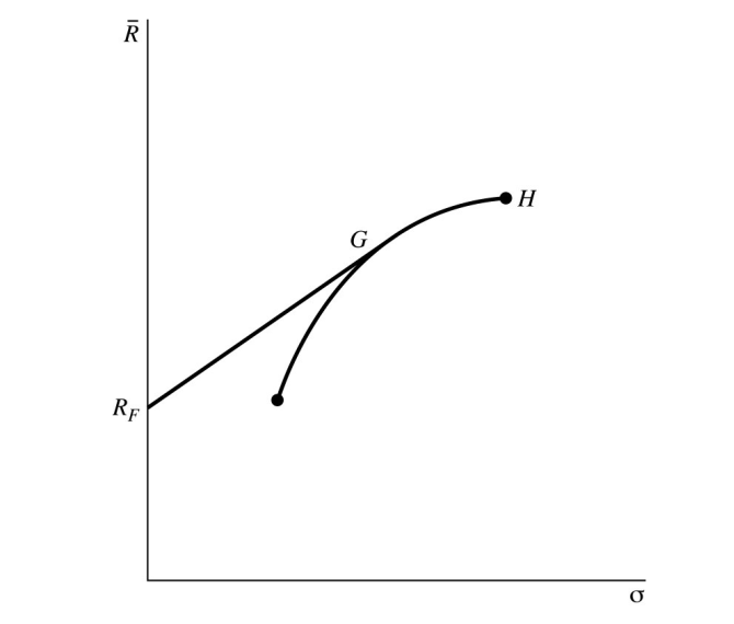
Consider the portfolios each having a different choice over the assets such that we cover all the following possibilities

[0, 0, 1]
[0, 0.1, 0.9]
[0.1, 0.1, 0.8]
.
.
[0.9, 0.1, 0]
[1, 0, 0]

三只股票分别是McDonald，Coca Cola和Microsoft, 时间为1991年１月１日到2001年１月１日

通过使用之前随笔中介绍的hist_stock_data获取.

if ~exist('stocks', 'var')
    stocks=hist_stock_data('01011991','01012001','KO','MCD','MSFT','frequency','wk');
    CocaCola = stocks(1);
    McDonalds = stocks(2);
    Microsoft = stocks(3);
end

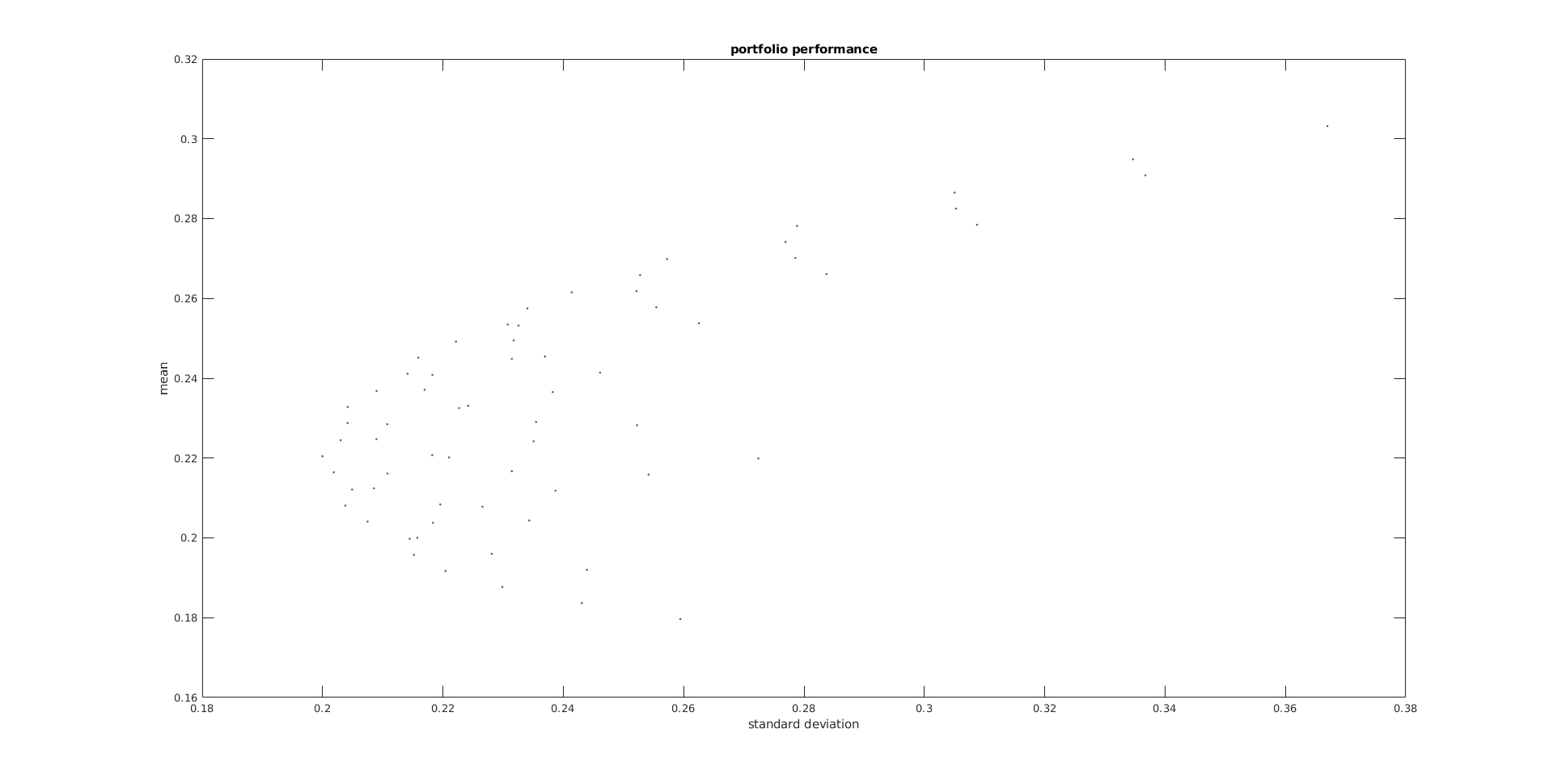
5.1 For each of the portfolios calculate the yearly mean and yearly standard deviation. Create a similar graph of mean against standard deviation.

% Caclualte log returns
CCLR  = log(CocaCola.AdjClose(2:end)./CocaCola.AdjClose(1:end-1) );
McLR  = log(McDonalds.AdjClose(2:end)./McDonalds.AdjClose(1:end-1) );
MicLR = log(Microsoft.AdjClose(2:end)./Microsoft.AdjClose(1:end-1) );

LogReturns = [ CCLR, McLR, MicLR ];

yearlymean = 52 * mean(LogReturns)';
yearlycov = 52 * cov(LogReturns)';

S = yearlycov;

% Now think about the portfolio 
% p is such that in total p_1 + p_2 + p_3 = 1 and we look at the following
% combinations of the form (0.1, 0.1, 0.8), (0.1, 0.2, 0.7) and so forth
x = zeros(67,0);
portfolios = [];
count = 1;
for i = 0:10
    for j = 0:10-i
        k = 10 - i - j;
            
        % assume the portfolio weights as x
        x = [i; j; k] / 10;
        portfolios = [ portfolios; x'];
        port_mean(count) = x' * yearlymean;
        port_var(count) = x' * S * x;
        port_std(count) = sqrt(port_var(count));
        count = count+1;
    end
end
np = count -1;
%  Plot portfolios
plot(port_std, port_mean, '.');

title ('portfolio performance');
xlabel('standard deviation');
ylabel('mean');

得到的Plot:

5.2 Which of the portfolios has the maximal mean

% highest expected return
max_r = find (port_mean == max(port_mean));

portfolios(max_r, :)

%pause;
hold on;
plot(port_std(max_r),port_mean(max_r), 'rx');

就是mean最高的点,(Y轴最高)

5.3 Which of the portfolios has the lowest standard deviation

% Lowest standatd deviation
min_std = find (port_std == min(port_std));


portfolios(min_std, :)

%pause;
hold on;
plot(port_std(min_std),port_mean(min_std), 'rx');

类似上步, x轴最小

5.4

Which of the portfolios has the highest ratio of mean to stdev ( μ_x/σ_x )? why is this portfolio interesting?

% Max slope (sharpe ratio)
max_slope = find (port_mean ./ port_std == max(port_mean ./ port_std));


%pause;
hold on;
plot(port_std(max_slope),port_mean(max_slope), 'rx');

portfolios(max_slope, :)
% Which portfolios dominate other portfolios

这个点对应的最佳投资, 为从mean轴对应var最小的点向曲线引出的切线与斜线的交点. 投资此处可以兼顾利润和风险

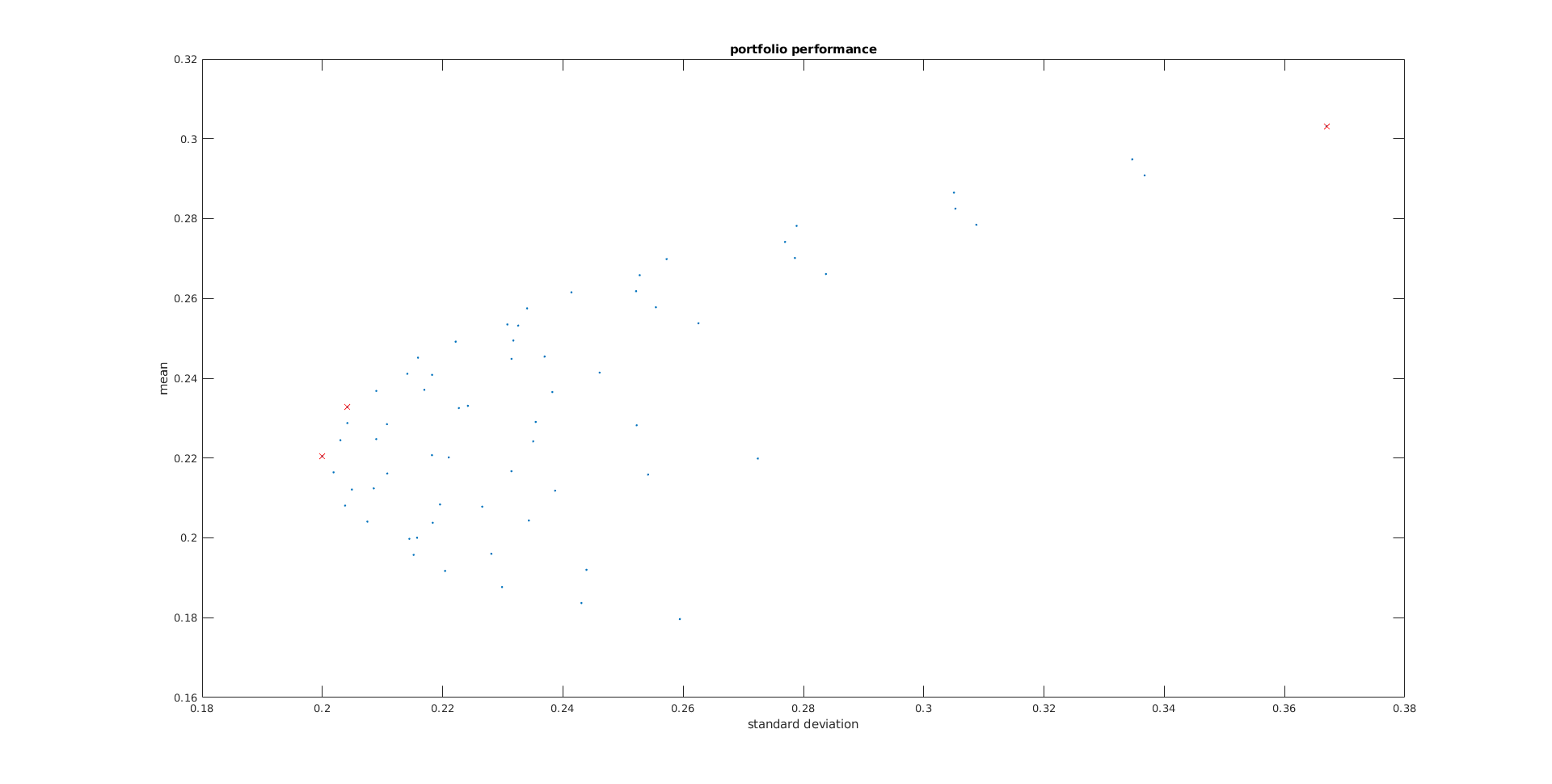
对应的最佳投资点:

使用MATLAB分析风险之下的投资分配方案

猜你喜欢