Mnist 数据集
Mnist是一个包含60000个训练样本和10000个测试样本的手写数字集合(下载地址)。通常,将60000个训练样本分为50000个实际训练样本和10000个交叉验证样本。每个样本是一副28*28的黑白图像,下面是典型图像。

为了方便处理,样本为2值图像(黑:0,白:1),每个样本被拉成一列(784),并且具有一个标号(0~9)。下面是读入数据集的代码:
import cPickle, gzip, numpy

# Load the dataset
f = gzip.open('mnist.pkl.gz', 'rb')
train_set, valid_set, test_set = cPickle.load(f)
f.close()
当实际使用数据时,通常将其分成很多块(随机梯度下降法,后文提到)。为了不用每次都从CPU内从中读取数据,再拿到GPU中做运算(这样会很慢),需要建立共享变量,这样每次GPU做运算时直接从GPU内从中读取数据就可以了。下面这段代码实现了数据共享,并取出数据中的一块。
import theano
import theano.tensor as T

def shared_dataset(data_xy):
    """ Function that loads the dataset into shared variables

    The reason we store our dataset in shared variables is to allow
    Theano to copy it into the GPU memory (when code is run on GPU).
    Since copying data into the GPU is slow, copying a minibatch everytime
    is needed (the default behaviour if the data is not in a shared
    variable) would lead to a large decrease in performance.
    """
    data_x, data_y = data_xy
    shared_x = theano.shared(numpy.asarray(data_x, dtype=theano.config.floatX))
    shared_y = theano.shared(numpy.asarray(data_y, dtype=theano.config.floatX))
    # When storing data on the GPU it has to be stored as floats
    # therefore we will store the labels as ``floatX`` as well
    # (``shared_y`` does exactly that). But during our computations
    # we need them as ints (we use labels as index, and if they are
    # floats it doesn't make sense) therefore instead of returning
    # ``shared_y`` we will have to cast it to int. This little hack
    # lets us get around this issue
    return shared_x, T.cast(shared_y, 'int32')

test_set_x, test_set_y = shared_dataset(test_set)
valid_set_x, valid_set_y = shared_dataset(valid_set)
train_set_x, train_set_y = shared_dataset(train_set)

batch_size = 500    # size of the minibatch

# accessing the third minibatch of the training set

data  = train_set_x[2 * batch_size: 3 * batch_size]
label = train_set_y[2 * batch_size: 3 * batch_size]
常用符号含义

训练数据
训练数据一般采用梯度下降法,先定义一个代价函数,代价函数的变量是网络的节点权重,求代价函数的导数,按导数的反方向更新代价函数,使代价函数达到极小值。此时对应的参数就是最佳权重,也就是最佳网络。
1.代价函数的选择
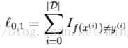
a.0-1损失
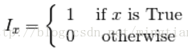
0-1损失,即预测正确,代价数为0,预测错误代价函数为1,D为训练数据集,则数学表示:
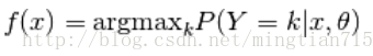
预测函数f的定义为选择当前样本对应概率最大的类别作为其分类标号 :
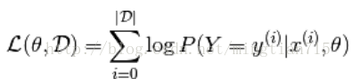
b.Negative Log-Likelihood(NLL)损失
因为0-1损失函数不可微分,计算困难。因此通常最大化对数极大似然函数(在极大似然函数基础做了对数,将概率相乘变为相加):
注意:Liklihood的最佳结果与正确分类个数最多是不相等的,即其与0-1损失不同,这是因为极大似然最大化的是概率和(预测结果和真实结果相同的概率)。
举个例子,假如有5个样本,其真实标号{0,1,0,1,0},假如有两种模型,其预测每个样例属于1个概率分别为{0.4,0.6,0.4,0.6,0.4}和{0.1,0.4,0.1,0.9,0.1}。第一种预测结果是全部正确,第二种预测结果第2个样例预测错误,但是对于似然估计来说,其代价函数是与概率相关,而非准确率相关,因此第二种结果对其来说是更优的结果。
通常习惯最小化,因此取-L作为代价函数,即NLL损失:

# NLL is a symbolic variable ; to get the actual value of NLL, this symbolic
# expression has to be compiled into a Theano function (see the Theano
# tutorial for more details)
NLL = -T.sum(T.log(p_y_given_x)[T.arange(y.shape[0]), y])
# note on syntax: T.arange(y.shape[0]) is a vector of integers [0,1,2,...,len(y)].
2.梯度下降法
有关梯度下降法和随机梯度下降法的原理就不叙述了,可以参看梯度下降介绍。
a.梯度下降法(GD)
# GRADIENT DESCENT

while True:
    loss = f(params)
    d_loss_wrt_params = ... # compute gradient
    params -= learning_rate * d_loss_wrt_params
    if <stopping condition is met>:
        return params
b.随机梯度下降法(SGD)
随机选择一个样本更新代价函数。
# STOCHASTIC GRADIENT DESCENT
for (x_i,y_i) in training_set:
                            # imagine an infinite generator
                            # that may repeat examples (if there is only a finite training set)
    loss = f(params, x_i, y_i)
    d_loss_wrt_params = ... # compute gradient
    params -= learning_rate * d_loss_wrt_params
    if <stopping condition is met>:
        return params
c.批量(Minibatch)随机梯度下降法(MSGD)
如果只针对一个样本更新代价函数的话,可能会使得代价函数出现较大波动,优化次数过多,一般是选择一定数量的样本。
for (x_batch,y_batch) in train_batches:
                            # imagine an infinite generator
                            # that may repeat examples
    loss = f(params, x_batch, y_batch)
    d_loss_wrt_params = ... # compute gradient using theano
    params -= learning_rate * d_loss_wrt_params
    if <stopping condition is met>:
        return params
样本数量的选择比较关键。只有样本数量较小时,增加数量才会减小更新过程中代价函数的波动,样本数量较多时,增加数目所能带来的改善很小,带来的更多的是计算时间的增大。本教程选择了B=20。
Theano中的实现:
# Minibatch Stochastic Gradient Descent

# assume loss is a symbolic description of the loss function given
# the symbolic variables params (shared variable), x_batch, y_batch;

# compute gradient of loss with respect to params
d_loss_wrt_params = T.grad(loss, params)

# compile the MSGD step into a theano function
updates = [(params, params - learning_rate * d_loss_wrt_params)]
MSGD = theano.function([x_batch,y_batch], loss, updates=updates)

for (x_batch, y_batch) in train_batches:
    # here x_batch and y_batch are elements of train_batches and
    # therefore numpy arrays; function MSGD also updates the params
    print('Current loss is ', MSGD(x_batch, y_batch))
    if stopping_condition_is_met:
        return params
防止过拟合
为了防止过拟合,通常要使用正则化方法,包括基于范数的正则化以及提前停止。
1.L1、L2范数正则化
此方法是在原代价函数基础上添加正则化项,使得整个网络权重系数分配相对平滑,不会出现某个权重系数过大。正则化项R(θ)是权重系数θ的函数。
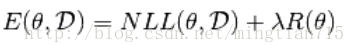
本教程中,R(θ)为:

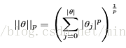
λ是控制正则化权重系数,||θ||p为p范数,通常选择p=1和p=2。实际优化过程中,就是寻找一个可以使得模型尽量拟合所有数据,但又使得权重系数平滑的平衡点。对应代码:
# symbolic Theano variable that represents the L1 regularization term
L1  = T.sum(abs(param))

# symbolic Theano variable that represents the squared L2 term
L2 = T.sum(param ** 2)

# the loss
loss = NLL + lambda_1 * L1 + lambda_2 * L2
2.提前停止
提前停止是一种通过交叉验证集来防止过拟合的方式。通常交叉验证集被我们看作是未来可能出现的数据样本,因此如果模型在很长时间内不能使得交叉验证集有着更好的拟合效果,甚至更差,此时应该停止优化。
如下面代码所示,简要解释一下过程:
patience代表最大优化次数
iter代表已优化次数
patience_increase代表patience的更新系数,如果发现交叉验证获得更好地结果,则有理由继续优化,可以通过下面这行代码增大patience。
patience = max(patience, iter * patience_increase)
improvement_threshold代表必须达到原代价函数的百分之多少才算有了改善,例如0.8,0.95。
validataion_frequence代表交叉验证的频率,毕竟不可能每次更新都交叉验证,那成训练集,不是交叉验证集了。
# early-stopping parameters
patience = 5000  # look as this many examples regardless
patience_increase = 2     # wait this much longer when a new best is
                              # found
improvement_threshold = 0.995  # a relative improvement of this much is
                               # considered significant
validation_frequency = min(n_train_batches, patience/2)
                              # go through this many
                              # minibatches before checking the network
                              # on the validation set; in this case we
                              # check every epoch

best_params = None
best_validation_loss = numpy.inf
test_score = 0.
start_time = time.clock()

done_looping = False
epoch = 0
while (epoch < n_epochs) and (not done_looping):
    # Report "1" for first epoch, "n_epochs" for last epoch
    epoch = epoch + 1
    for minibatch_index in range(n_train_batches):

        d_loss_wrt_params = ... # compute gradient
        params -= learning_rate * d_loss_wrt_params # gradient descent

        # iteration number. We want it to start at 0.
        iter = (epoch - 1) * n_train_batches + minibatch_index
        # note that if we do `iter % validation_frequency` it will be
        # true for iter = 0 which we do not want. We want it true for
        # iter = validation_frequency - 1.
        if (iter + 1) % validation_frequency == 0:

            this_validation_loss = ... # compute zero-one loss on validation set

            if this_validation_loss < best_validation_loss:

                # improve patience if loss improvement is good enough
                if this_validation_loss < best_validation_loss * improvement_threshold:

                    patience = max(patience, iter * patience_increase)
                best_params = copy.deepcopy(params)
                best_validation_loss = this_validation_loss

        if patience <= iter:
            done_looping = True
            break

# POSTCONDITION:
# best_params refers to the best out-of-sample parameters observed during the optimization
注意:如果patience次数没达到就运行完了整个数据集,则返回数据集的开始重复过程。另validation_frequence必须小于patience,并且整个优化过程至少进行2次交叉验证(即patience/2的由来)。
至此,本小节结束了,主要讲述了如何将数据保存到GPU中以便后续运算,以及神经网络的基础优化和抑制过拟合方法等。