前言:pip install -U scikit-learn安装sklearn模块
文章目录
x[:,0]和x[:,1] 理解和实例解析
x[m,n]是通过numpy库引用数组或矩阵中的某一段数据集的一种写法,
m代表第m维,n代表m维中取第几段特征数据。
通常用法:
x[:,n]或者x[n,:]
x[:,n]表示在全部数组(维)中取第n个数据,直观来说,x[:,n]就是取所有集合的第n个数据,
举例说明:
x[:,0]
import numpy as np

X = np.array([[0,1],[2,3],[4,5],[6,7],[8,9],[10,11],[12,13],[14,15],[16,17],[18,19]])
print X[:,0]
结果:
[ 0  2  4  6  8 10 12 14 16 18]

x[:,1]
import numpy as np

X = np.array([[0,1],[2,3],[4,5],[6,7],[8,9],[10,11],[12,13],[14,15],[16,17],[18,19]])
print X[:,1]
结果为:
[ 1  3  5  7  9 11 13 15 17 19]
扩展用法
x[:,m:n],即取所有数据集的第m到n-1列数据
例:输出X数组中所有行第1到2列数据
X = np.array([[0,1,2],[3,4,5],[6,7,8],[9,10,11],[12,13,14],[15,16,17],[18,19,20]])
print X[:,1:3]
结果为:
[[ 1  2]
 [ 4  5]
 [ 7  8]
 [10 11]
 [13 14]
 [16 17]
 [19 20]]
load_boston数据集
通过print (data["DESCR"])查看数据集的详细介绍
Signature: load_boston(return_X_y=False)
Docstring:
Load and return the boston house-prices dataset (regression).

==============   ==============
Samples total               506
Dimensionality               13
Features         real, positive
Targets           real 5. - 50.
==============   ==============

Read more in the :ref:`User Guide <boston_dataset>`.

Parameters
----------
return_X_y : boolean, default=False.
    If True, returns ``(data, target)`` instead of a Bunch object.
    See below for more information about the `data` and `target` object.

    .. versionadded:: 0.18

Returns
-------
data : Bunch
    Dictionary-like object, the interesting attributes are:
    'data', the data to learn, 'target', the regression targets,
    'DESCR', the full description of the dataset,
    and 'filename', the physical location of boston
    csv dataset (added in version `0.20`).

(data, target) : tuple if ``return_X_y`` is True

    .. versionadded:: 0.18

Notes
-----
    .. versionchanged:: 0.20
        Fixed a wrong data point at [445, 0].

Examples
--------
>>> from sklearn.datasets import load_boston
>>> X, y = load_boston(return_X_y=True)
>>> print(X.shape)
zip函数
zip函数接受任意多个(包括0个和1个)序列作为参数,返回一个tuple列表。具体意思不好用文字来表述,直接看示例:
1.
x = [1, 2, 3]

y = [4, 5, 6]

z = [7, 8, 9]

xyz = zip(x, y, z)

print (xyz)
结果为:
[(1, 4, 7), (2, 5, 8), (3, 6, 9)]
x = [1, 2, 3]
y = [4, 5, 6, 7]
xy = zip(x, y)
print (xy)
结果:
[(1, 4), (2, 5), (3, 6)]

从这个结果可以看出zip函数的长度处理方式。
x = [1, 2, 3]
x = zip(x)
print (x)
运行的结果是:
[(1,), (2,), (3,)]
从这个结果可以看出zip函数在只有一个参数时运作的方式。
x = [1, 2, 3]
y = [4, 5, 6]
z = [7, 8, 9]
xyz = zip(x, y, z)
u = zip(*xyz)
print (u)
运行的结果是:
[(1, 2, 3), (4, 5, 6), (7, 8, 9)]
一般认为这是一个unzip的过程,它的运行机制是这样的:
在运行zip(*xyz)之前,xyz的值是:[(1, 4, 7), (2, 5, 8), (3, 6, 9)]
那么,zip(*xyz) 等价于 zip((1, 4, 7), (2, 5, 8), (3, 6, 9))
所以,运行结果是:[(1, 2, 3), (4, 5, 6), (7, 8, 9)],python中的*号 删除可以看这里
注:在函数调用中使用*list/tuple的方式表示将list/tuple分开,作为位置参数传递给对应函数(前提是对应函数支持不定个数的位置参数)
x = [1, 2, 3]
r = zip(* [x] * 3)
print(r)
运行的结果是:

[(1, 1, 1), (2, 2, 2), (3, 3, 3)]

它的运行机制是这样的:
[x]生成一个列表的列表,它只有一个元素x
[x] * 3生成一个列表的列表,它有3个元素,[x, x, x]
zip(* [x] * 3)的意思就明确了,zip(x, x, x)
关于loss函数理解
https://www.cnblogs.com/guoyaohua/p/9217206.html
First-Method: Random generation: get best k and best b
Python中可以用如下方式表示正负无穷:float("inf"), float("-inf")
from sklearn.datasets import load_boston
import matplotlib.pyplot as plt
import random
data = load_boston()
X, y = data['data'], data['target']
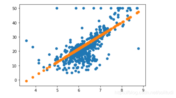
# 生成面积与房价的散点图
def draw_rm_and_price():
plt.scatter(X[:, 5], y)
def price(rm, k, b):
"""f(x) = k * x + b"""
return k * rm + b
# 房价
X_rm = X[:, 5]
k = random.randint(-100, 100)
b = random.randint(-100, 100)
# price_by_random_k_and_b = [price(r, k, b) for r in X_rm]
# print(price_by_random_k_and_b)
# plt.scatter(X[:, 5], y)
# plt.scatter(X_rm, price_by_random_k_and_b)
# plt.show()
# to evaluate the performance
def loss(y, y_hat):
return sum((y_i - y_hat_i) ** 2 for y_i, y_hat_i in zip(list(y), list(y_hat))) / len(list(y))
trying_times = 2000
min_loss = float('inf')
best_k, best_b = None, None
for i in range(trying_times):
k = random.random() * 200 - 100
b = random.random() * 200 - 100
price_by_random_k_and_b = [price(r, k, b) for r in X_rm]
current_loss = loss(y, price_by_random_k_and_b)
if current_loss < min_loss:
min_loss = current_loss
best_k, best_b = k, b
print('When time is : {}, get best_k: {} best_b: {}, and the loss is: {}'.format(i, best_k, best_b, min_loss))
X_rm = X[:, 5]
k = best_k
b = -best_b
price_by_random_k_and_b = [price(r, k, b) for r in X_rm]
draw_rm_and_price()
plt.scatter(X_rm, price_by_random_k_and_b)
plt.show()
2nd-Method: Direction Adjusting
from sklearn.datasets import load_boston
import matplotlib.pyplot as plt
import random
data = load_boston()
X, y = data['data'], data['target']
# 生成面积与房价的散点图
def draw_rm_and_price():
plt.scatter(X[:, 5], y)
def price(rm, k, b):
"""f(x) = k * x + b"""
return k * rm + b
# 房价
X_rm = X[:, 5]
# to evaluate the performance
def loss(y, y_hat): # to evaluate the performance
return sum((y_i - y_hat_i)**2 for y_i, y_hat_i in zip(list(y), list(y_hat))) / len(list(y))
trying_times = 20000
min_loss = float('inf')
best_k, best_b = random.random() * 200 - 100, random.random() * 200 - 100
direction =[
(+1, -1), # first element: k's change direction, second element: b's change direction
(+1, +1),
(-1, -1),
(-1, +1),
]
next_direction = random.choice(direction)
scalar = 0.05
update_time = 0
for i in range(trying_times):
k_direction, b_direction = next_direction
current_k, current_b = best_k + k_direction * scalar, best_b + b_direction * scalar
price_by_k_and_b = [price(r, current_k, current_b) for r in X_rm]
current_loss = loss(y, price_by_k_and_b)
# performance became better
if current_loss < min_loss:
min_loss = current_loss
best_k, best_b = current_k, current_b
next_direction = next_direction
update_time += 1
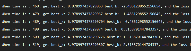
if update_time % 10 ==0:
print(
'When time is : {}, get best_k: {} best_b: {}, and the loss is: {}'.format(i, best_k, best_b, min_loss))
else:
next_direction = random.choice(direction)
X_rm = X[:,5]
k, b = best_k, best_b
price_by_random_k_and_b = [price(r, k, b) for r in X_rm]
draw_rm_and_price()
plt.scatter(X_rm, price_by_random_k_and_b)
plt.show()
如果我们想得到更快的更新,在更短的时间内获得更好的结果,我们需要一件事情:
找对改变的方向
如何找对改变的方向呢?
2nd-method: 监督让他变化–> 监督学习
3nd-method梯度下降
from sklearn.datasets import load_boston
import matplotlib.pyplot as plt
import random

data = load_boston()
X, y = data['data'], data['target']


# 生成面积与房价的散点图
def draw_rm_and_price():
    plt.scatter(X[:, 5], y)


def price(rm, k, b):
    """f(x) = k * x + b"""
    return k * rm + b


# 房价
X_rm = X[:, 5]


# to evaluate the performance
def loss(y, y_hat):  # to evaluate the performance
    return sum((y_i - y_hat_i) ** 2 for y_i, y_hat_i in zip(list(y), list(y_hat))) / len(list(y))


def partial_k(x, y, y_hat):
    n = len(y)
    gradient = 0
    for x_i, y_i, y_hat_i in zip(list(x), list(y), list(y_hat)):
        gradient += (y_i - y_hat_i) * x_i

    return -2 / n * gradient


def partial_b(x, y, y_hat):
    n = len(y)
    gradient = 0
    for y_i, y_hat_i in zip(list(y), list(y_hat)):
        gradient += (y_i - y_hat_i)
    return -2 / n * gradient


trying_times = 100000

X, y = data['data'], data['target']

min_loss = float('inf')

current_k = random.random() * 200 - 100
current_b = random.random() * 200 - 100
best_k = random.random() * 200 - 100
best_b = random.random() * 200 - 100
learning_rate = 1e-03
update_time = 0
for i in range(trying_times):
    price_by_k_and_b = [price(r, current_k, current_b) for r in X_rm]
    current_loss = loss(y, price_by_k_and_b)
    if current_loss < min_loss:
        min_loss = current_loss
        if i % 50 == 0:
            print(
                'When time is : {}, get best_k: {} best_b: {}, and the loss is: {}'.format(i, best_k, best_b, min_loss))

        k_gradient = partial_k(X_rm, y, price_by_k_and_b)
        b_gradient = partial_b(X_rm, y, price_by_k_and_b)
        # 如果k大于0说明在增加要防止增加就要让k减小,k小于0也是这样所以前面加上-1
        current_k = current_k + (-1 * k_gradient) * learning_rate
        current_b = current_b + (-1 * b_gradient) * learning_rate

X_rm = X[:, 5]
k, b = current_k, current_b
price_by_random_k_and_b = [price(r, k, b) for r in X_rm]
draw_rm_and_price()
plt.scatter(X_rm, price_by_random_k_and_b)
plt.show()