tensorflow实现手写数字验证码识别

手写数字识别这个例子是学tensorflow必经的小练习喔

本次使用到的是网上的mnist数据集，官网下载速度极慢，这里附上百度云下载链接： https://pan.baidu.com/s/1O9sfNiYswBq6uKLioyVXAw 提取码: 1965

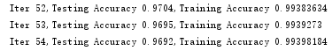
话不多说来个正确率的图，测试集正确率96%

啥？看着不好看？没看到过程？莫急，看下图，tensorboard可视化，多帅喔。

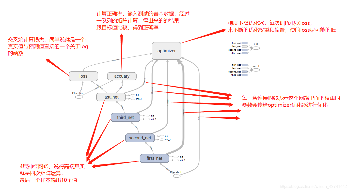
这是网络的结构图

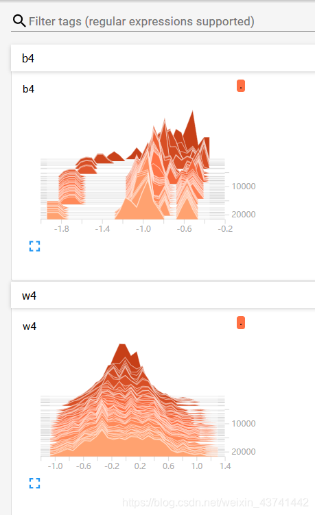
训练过程中的数据的变化

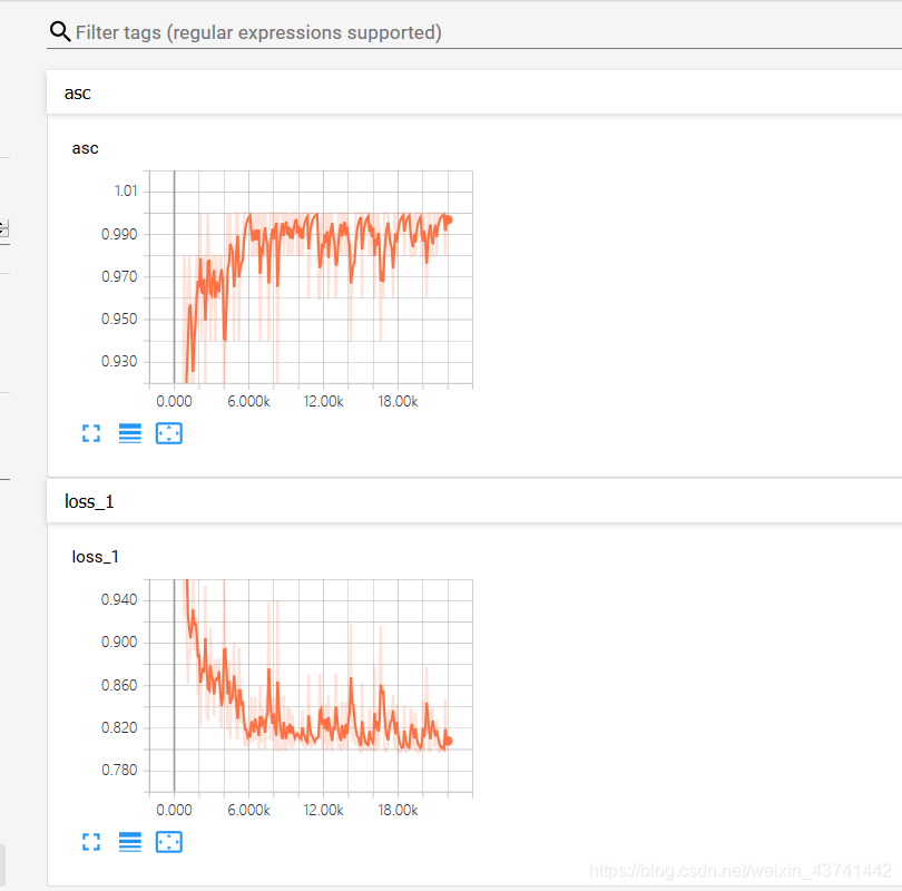
图中可以看到asc（正确率）在随着训练不断的上升，loss损失值也在不断的下降，其中用到的

下面是code部分，大部分内容可以看代码

创建一个简单的神经网络

# 这里所说的神经网络就是一些矩阵相乘，还要偏置的相加，最后保证输出10个值，因为手写数字只有10个类别
# 可以自行改一下里面中间层的神经元个数之类的，不过要注意确保可以矩阵相乘的条件
# 里面你可以加一层，两层也可以的，注意输出矩阵的格式呀求就好
# 就好比如：输入的为[None, 784], 因为图片有784个像素，也就是有784个特征，
#所以第一层的权重必须是是 [784, 神经元的个数]，偏置则是跟神经元个数一样就行了。

# coding: utf-8
import tensorflow as tf
from tensorflow.examples.tutorials.mnist import input_data

# 载入数据集
mnist = input_data.read_data_sets("../../tensorflow_code/mnist/", one_hot=True)

# 每个批次的大小
batch_size = 50
# 计算一共有多少个批次
n_batch = mnist.train.num_examples // batch_size

# 定义两个placeholder
x = tf.placeholder(tf.float32, [None, 784])
y = tf.placeholder(tf.float32, [None, 10])

# 这个可以设置有多少神经元在工作
# keep_prob = tf.placeholder(tf.float32)

with tf.variable_scope("first_net"):
    # 创建一个简单的神经网络，
    # 所谓的神经网络就是一些矩阵相乘，还要偏置的相加，最后保证输出10个值，因为手写数字只有10个类别
    # 可以自行改一下里面中间层的神经元个数之类的，不过要注意确保可以矩阵相乘的条件
    # 里面你可以加一层，两层也可以的，注意输出矩阵的格式呀求就好
    # 就好比如：输入的为[None, 784], 因为图片有784个像素，也就是有784个特征，
    #所以第一层的权重必须是是 [784, 神经元的个数]，偏置则是跟神经元个数一样就行了。
    
    W1 = tf.Variable(tf.random_normal([784, 50], stddev=0.1))
    b1 = tf.Variable(tf.zeros([50]))
    prediction1 = tf.nn.tanh(tf.matmul(x, W1) + b1)
    
    # 设置神经元的在训练的工作的比例，设置后，训练的数据集拿来测试的准确率跟测试集的差不多，
    # 如果不开，每个神经元都在训练，训练集的测试结果达到99，测试集的测试结果只有97
    # 在数据量少的时候体会不到重要，再使用goolenet或者Alexnet的时候，几百w的数据就非常明显了
    # L1_drop = tf.nn.dropout(prediction1, keep_prob)
    L1_drop = prediction1
    
    # 第一层输出的数据的类型为： [n个样本，784]*[784, 50个神经元]+[50个偏置值] = [n个样本, 50]
    #也就是说 一个神经元就输出一个值，下面类似
    
with tf.variable_scope("second_net"):
    W2 = tf.Variable(tf.random_normal([50, 50], stddev=0.1))
    b2 = tf.Variable(tf.zeros([50]))
    prediction2 = tf.nn.tanh(tf.matmul(L1_drop, W2) + b2)
    # L2_drop = tf.nn.dropout(prediction2, keep_prob)
    L2_drop = prediction2
with tf.variable_scope("third_net"):
    W3 = tf.Variable(tf.random_normal([50, 50], stddev=0.1))
    b3 = tf.Variable(tf.zeros([50]))
    prediction3 = tf.nn.tanh(tf.matmul(L2_drop, W3) + b3)
    # L3_drop = tf.nn.dropout(prediction3, keep_prob)
    L3_drop = prediction3
with tf.variable_scope("last_net"):
    W4 = tf.Variable(tf.zeros([50, 10]))
    b4 = tf.Variable(tf.zeros([10]))
    prediction = tf.nn.tanh(tf.matmul(L3_drop, W4) + b4)
# L4_drop = tf.nn.dropout(prediction3, keep_prob)


with tf.variable_scope("loss"):
    # 二次代价函数
    # loss = tf.reduce_mean(tf.square(y - prediction))
    # 使用交叉商损失计算损失，效果会比上面的方差要好
    loss = tf.reduce_mean(tf.nn.softmax_cross_entropy_with_logits(labels=y, logits=prediction))

with tf.variable_scope("optimizer"):
    # 使用梯度下降法
    train_step = tf.train.GradientDescentOptimizer(0.15).minimize(loss)

# 初始化变量
init = tf.global_variables_initializer()

with tf.variable_scope("accuary"):
    # 结果存放在一个布尔型列表中
    correct_prediction = tf.equal(tf.argmax(y, 1), tf.argmax(prediction, 1))  # argmax()返回一维张量中最大的值所在的位置
    
    # 求准确率
    # reduce_mean： 求这个张量里面的值的平均值，如：[1，0，0，1]，结果就是0.4
    # cast：改变数据的类型为float32
    accuracy = tf.reduce_mean(tf.cast(correct_prediction, tf.float32))

# 收集变量， 单个的数字值变量
tf.summary.scalar("loss", loss)
tf.summary.scalar("asc", accuracy)

# 高维度数据收集，这里就收集最后一层好了
# tf.summary.histogram("w1", W1)
# tf.summary.histogram("b1", b1)
# tf.summary.histogram("weights", W2)
# tf.summary.histogram("biases", b2)
# tf.summary.histogram("weights", W3)
# tf.summary.histogram("biases", b3)
tf.summary.histogram("w4", W4)
tf.summary.histogram("b4", b4)


# 定义一个初始化变量op
init_op = tf.global_variables_initializer()

# 定义一个合并变量的OP, 用于后面将变量不断的加入到event里面
merge = tf.summary.merge_all()


with tf.Session() as sess:
    sess.run(init)

    # 建立event事件, filewriter用于每一步保存变量的值到event里面去
    filewriter = tf.summary.FileWriter("./model/", graph=sess.graph)
    # 用于记录训练的批次
    i += 1

    for epoch in range(20):
        for batch in range(n_batch):
            # 获取一批次的训练数据
            batch_xs, batch_ys = mnist.train.next_batch(batch_size)
            # 传入数据进行训练
            # sess.run(train_step, feed_dict={x: batch_xs, y: batch_ys, keep_prob: 0.7})
            sess.run(train_step, feed_dict={x: batch_xs, y: batch_ys})

        # 每训练100个批次写入一次W，b，loss，accuracy的值，用于tensorboard 画图
            if i % 100 == 0:
                summary = sess.run(merge, feed_dict={x: batch_xs, y: batch_ys})

                # i就相当于画图的时候的横坐标
                filewriter.add_summary(summary, i)

        # test_acc = sess.run(accuracy, feed_dict={x: mnist.test.images, y: mnist.test.labels, keep_prob: 1.0})
        # train_acc = sess.run(accuracy, feed_dict={x: mnist.train.images, y: mnist.train.labels, keep_prob: 1.0})
        test_acc = sess.run(accuracy, feed_dict={x: mnist.test.images, y: mnist.test.labels})
        train_acc = sess.run(accuracy, feed_dict={x: mnist.train.images, y: mnist.train.labels})
        print("Iter " + str(epoch) + ",Testing Accuracy " + str(test_acc) + ",Training Accuracy " + str(train_acc))

小结： 这次分享的主要是比较基础的手写数字的识别，写得可能不是很详细，不过可以自行看下注释，以及自己修改一些参数可以帮助理解，对于tensorboard不能显示出图的问题，会在我的另一篇博客中提到，欢迎多多指教。