最近一月在郫县大数据中心实训,实训的项目包括Python数据处理和Spark ML,我选的实训的结题项目为MNIST手写数字识别项目,一来是对学的Python知识进行总结,二来是对机器学习进行一个入门,特整理博客,梳理一下思路。
拿到这个题目,加上之前对于机器学习理论知识的学习,首先想到的是使用Tensorflow框架进行编写,因为Python实现较为多,也较为顺手,几乎不会遇到一些未知和无关的错误。
这里实现一个基于Tensorflow的MNIST手写数字识别及Web验证的实现,也就是包括数据处理、机器学习的训练、再到测试集的验证、再实现一个前端在线测试,就是手动画一个数字,利用API,使用训练好的模型进行测试,查看效果。
我跟的教程为官方教程。所用技术为Tensorflow + Numpy+Flask。采用的模型包括regression回归 和convolution卷积 两种。
此处不再说明如何配环境了,对于这些包的安装都是cmd中pip install命令,IDE采用PyCharm
pip install tensorflow
pip install numpy
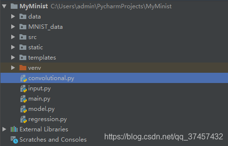
pip install flask关于本项目的架构为
---MyMnist //项目总目录
------data //训练得到的模型文件的目录
------MNIST_data //MNIST数据集:训练集和测试集,一共四个文件
------input.py //用于在项目中读取数据集
------model.py //定义模型(卷积和回归)的函数
------convolutional.py //卷积的具体实现:训练和测试
------regression.py //回归的具体实现:训练和测试
------main.py//为前端提供一个接口,用于运行前端和数据传送
------其他网页前端文件夹(src、static、templates)
1.首先导入MNIST数据集。数据集可以手动导入,也可以利用Tf自带的datasets进行导入,前者可以自己去下载,建一个包装进去,然后就会自动解压识别。我这里使用的是后者,当时公司断网,就又手动导入了。
input.py
from __future__ import absolute_import
from __future__ import division
from __future__ import print_function

import tensorflow
import gzip
import os
import tempfile

import numpy
from six.moves import urllib
from six.moves import xrange

from tensorflow.contrib.learn.python.learn.datasets.mnist import  read_data_sets
input.py负责数据集的导入,以及必要包的导入。
这里的read_data_sets会被后边经常用到,调用来读取数据集。mnist在tf中内置
在input写好以后,在新建的py文件中,先import input 再data=input.read_data_sets即可将数据集下载、解压、赋给data
接下来,构造网络模型model.py
import tensorflow as tf

#y=wx+b
def regression(x):
    W = tf.Variable(tf.zeros([784,10]),name="W")  #all is 0 定义权重w,784*10的图像
    b=tf.Variable(tf.zeros([10]),name="b") #定义偏移量b
    y=tf.nn.softmax(tf.matmul(x,W)+b) #定义y

    return y, [W, b]

def convolutional(x, keep_prob):
    def conv2d(x, W):  # 卷积层
        return tf.nn.conv2d(x,W,strides=[1, 1, 1, 1], padding='SAME')

    def max_pool_2x2(x):  # 池化层
        return tf.nn.max_pool(x, ksize=[1, 2, 2, 1], strides=[1, 2, 2, 1], padding='SAME')

    def weight_variable(shape):  # 定义权重
        initial = tf.truncated_normal(shape, stddev=0.1)
        return tf.Variable(initial)

    def bias_variable(shape):  # 定义bias
        initial = tf.constant(0.1,shape=shape)
        return tf.Variable(initial)
# 第一层
    x_image = tf.reshape(x,[-1, 28, 28, 1])
    W_conv1 = weight_variable([5, 5, 1, 32])
    b_conv1 = bias_variable([32])
    h_conv1 = tf.nn.relu(conv2d(x_image, W_conv1)+b_conv1)
    h_pool1 = max_pool_2x2(h_conv1)

# 第二层
    W_conv2 = weight_variable([5, 5, 32, 64])
    b_conv2 = bias_variable([64])
    h_conv2 = tf.nn.relu(conv2d(h_pool1, W_conv2) + b_conv2)
    h_pool2 = max_pool_2x2(h_conv2)

#全连接层
    W_fc1 = weight_variable([7*7*64, 1024])
    b_fc1 = bias_variable([1024])
    h_pool2_flat = tf.reshape(h_pool2,[-1, 7*7*64])
    h_fc1=tf.nn.relu(tf.matmul(h_pool2_flat, W_fc1)+b_fc1)

    h_fc1_drop = tf.nn.dropout(h_fc1, keep_prob)

    W_fc2=weight_variable([1024,10])
    b_fc2=bias_variable([10])
    y = tf.nn.softmax(tf.matmul(h_fc1_drop,W_fc2)+b_fc2)

    return y, [W_conv1, b_conv1, W_conv2, b_conv2, W_fc1, b_fc1, W_fc2, b_fc2]
首先是对回归模型的函数的定义
#y=wx+b
def regression(x):
    W = tf.Variable(tf.zeros([784,10]),name="W")  #all is 0 定义权重w,784*10个0
    b=tf.Variable(tf.zeros([10]),name="b") #定义偏移量b
    y=tf.nn.softmax(tf.matmul(x,W)+b) #定义y

    return y, [W, b]
这一段主要就是实现 y=wx+b
先定义权重w 偏移量b 然后定义y与w x和b的关系,其中Softmax函数,或称归一化指数函数,是逻辑函数的一种推广。
W = tf.Variable(tf.zeros([784,10]),name="W") #定义权重为 784*10个值,并全部赋值为0
为什么是784*10呢?因为这是回归模型,如图所示,输入为28*28的图像,也就是输入为784个变量,而输出为0-9这十个数。
或者根据y=wx+b对应的矩阵模型,输入x为784行1列的矩阵、w为784行10列的矩阵、b为10行1列的矩阵,y也是10行1列。
矩阵相乘是左行乘右列,w乘x就变成了10行一列,正好与b相匹配。
如图所示(盗的图)

接着是卷积函数的定义
def convolutional(x, keep_prob):
    def conv2d(x, W):  # 卷积层
        return tf.nn.conv2d(x,W,strides=[1, 1, 1, 1], padding='SAME')

    def max_pool_2x2(x):  # 池化层
        return tf.nn.max_pool(x, ksize=[1, 2, 2, 1], strides=[1, 2, 2, 1], padding='SAME')

    def weight_variable(shape):  # 定义权重
        initial = tf.truncated_normal(shape, stddev=0.1)
        return tf.Variable(initial)

    def bias_variable(shape):  # 定义bias
        initial = tf.constant(0.1,shape=shape)
        return tf.Variable(initial)
# 第一层
    x_image = tf.reshape(x,[-1, 28, 28, 1])
    W_conv1 = weight_variable([5, 5, 1, 32])
    b_conv1 = bias_variable([32])
    h_conv1 = tf.nn.relu(conv2d(x_image, W_conv1)+b_conv1)
    h_pool1 = max_pool_2x2(h_conv1)

# 第二层
    W_conv2 = weight_variable([5, 5, 32, 64])
    b_conv2 = bias_variable([64])
    h_conv2 = tf.nn.relu(conv2d(h_pool1, W_conv2) + b_conv2)
    h_pool2 = max_pool_2x2(h_conv2)

#全连接层
    W_fc1 = weight_variable([7*7*64, 1024])
    b_fc1 = bias_variable([1024])
    h_pool2_flat = tf.reshape(h_pool2,[-1, 7*7*64])
    h_fc1=tf.nn.relu(tf.matmul(h_pool2_flat, W_fc1)+b_fc1)

    h_fc1_drop = tf.nn.dropout(h_fc1, keep_prob)

    W_fc2=weight_variable([1024,10])
    b_fc2=bias_variable([10])
    y = tf.nn.softmax(tf.matmul(h_fc1_drop,W_fc2)+b_fc2)
return y, [W_conv1, b_conv1, W_conv2, b_conv2, W_fc1, b_fc1, W_fc2, b_fc2]
本项目的卷积神经网络包括三层
第一层内有 卷积层、池化层,先卷积再池化,激活函数是relu
第二层内有 卷积层、池化层,先卷积再池化,激活函数是relu
第三层为全连接层,将前两层的参数进行全连接。激活函数是softmax
这部分后面的内容主要是对所用到的参数进行声明和定义,最后将这部分参数作为返回值进行返回。
接下来是进行两种算法的实现
regression.py 这部分具体实现回归算法。
import input
import os
import model
import tensorflow as tf


#读取数据集
data=input.read_data_sets("MNIST_data",one_hot=True)

# 建立回归模型,定义此次要用到的x 将x传入上面实现的regression函数中对y等进行赋值。
with tf.variable_scope("regression"):
    x=tf.placeholder(tf.float32, [None, 784])  #占位符
    y, variables = model.regression(x)

# 设定训练的一系列参数
y_=tf.placeholder("float",[None,10])
# 定义交叉熵
cross_entropy=-tf.reduce_sum(y_ * tf.log(y))
# 定义训练的步长,采用优化器
train_step=tf.train.GradientDescentOptimizer(0.01).minimize(cross_entropy)

correct_prediction=tf.equal(tf.arg_max(y,1),tf.argmax(y_,1))
# 准确度
accuracy = tf.reduce_mean(tf.cast(correct_prediction,tf.float32))

# 用来保存所有参数
saver =tf.train.Saver(variables)

#开始训练
with tf.Session() as sess:
    sess.run(tf.global_variables_initializer())
    for _ in range(1000):
        batch_xs, batch_ys = data.train.next_batch(100)
        sess.run(train_step, feed_dict={x:batch_xs, y_:batch_ys})

#测试集、测试准确率
    print((sess.run(accuracy,feed_dict={x:data.test.images, y_:data.test.labels})))

#保存模型到ckpt
    path=saver.save(
        sess, os.path.join(os.path.dirname(__file__), 'data', 'regression.ckpt'), # 存到ckpt文件里
        write_meta_graph=False, write_state=False)  # 不存到图里

    print("Saved:", path)
convolutional.py 这部分具体实现卷积神经网络
import os
import model
import tensorflow as tf
import input

data = input.read_data_sets('MNIST_data',one_hot=True)

#model
with tf.variable_scope("convolutional"):
    x = tf.placeholder(tf.float32,[None,784], name='x')
    keep_prob = tf.placeholder(tf.float32)
    y, variables = model.convolutional(x, keep_prob)

#train
y_ = tf.placeholder(tf.float32, [None, 10], name='y')
cross_entropy = -tf.reduce_sum(y_ * tf.log(y))
train_step = tf.train.AdamOptimizer(1e-4).minimize(cross_entropy)
correct_prediction = tf.equal(tf.argmax(y, 1), tf.argmax(y_, 1))
accuracy = tf.reduce_mean(tf.cast(correct_prediction,tf.float32))

saver = tf.train.Saver(variables)

with tf.Session() as sess:
    merged_summary_op = tf.summary.merge_all()
    summary_writer = tf.summary.FileWriter('/tmp/mnist_log/1', sess.graph)
    summary_writer.add_graph(sess.graph)  # 将它的图保存起来
    sess.run(tf.global_variables_initializer())

    for i in range(20000): # 设置训练两万次
        batch = data.train.next_batch(50)
        if i % 100 == 0:  # 每100次对准确率进行打印
            train_accuracy = accuracy.eval(feed_dict={x: batch[0], y_: batch[1], keep_prob: 1.0})
            print("Step %d, training accuracy %g" % (i, train_accuracy))
        sess.run(train_step,feed_dict={x: batch[0], y_: batch[1],keep_prob: 0.5 })

    # 测试
    print(sess.run(accuracy,feed_dict={x: data.test.images, y_: data.test.labels, keep_prob: 1.0}))

    path = saver.save(
        sess, os.path.join(os.path.dirname(__file__), 'data', 'convolutional.ckpt'),
        write_meta_graph = False, write_state=False)

    print("Saved:", path)
这部分主要是对两种回归函数进行训练、测试。
接下来,我们对regression.py和convolutional.py进行运行,进行训练,并且得到模型。
这里要注意的是,先建好data文件夹,不然会报错。
将前端代码编写好以后导入项目中,以完成前端逻辑并展示。
然后进行前端接口设计。其实也就是获取网页前端的输入(一幅图片),进行处理以后,分散到格子中,转化为坐标,然后传回服务器,利用API与已经训练好的模型进行比较,并返回结果。
main.py
import numpy as np
import tensorflow as tf
from flask import Flask,jsonify, render_template, request

import model

x=tf.placeholder("float",[None, 784])
sess= tf.Session()

with tf.variable_scope("regression"):
    y1, variables = model.regression(x)
saver = tf.train.Saver(variables)
saver.restore(sess,"data/regression.ckpt")

with tf.variable_scope("convolutional"):
    keep_prob = tf.placeholder("float")
    y2, variables = model.convolutional(x, keep_prob)
saver = tf.train.Saver(variables)
saver.restore(sess,"data/convolutional.ckpt")

def regression(input):
    return sess.run(y1, feed_dict={x: input}).flatten().tolist()

def convolutional(input):
    return sess.run(y2,feed_dict={x:input,keep_prob:1.0}).flatten().tolist()

app=Flask(__name__)
@app.route('/api/mnist',methods=['post'])
def mnist():
    input = ((255 - np.array(request.json, dtype=np.uint8))/255.0).reshape(1,784)
    output1 = regression(input)
    output2 = convolutional(input)

    return jsonify(results=[output1, output2])

@app.route('/')
def main():
    return render_template('index.html')

if __name__ =='__main__':
    app.debug = True
    app.run(host='127.0.0.1',port=8000)
接下来运行main.py即可开启服务器,使用chrome浏览器即可查看。


可以看出,卷积神经网络实现的更准确一点。
