自编码网络的使用方法 -- 栈式自编码神经网络 SA

栈式自编码神经网络（Stacked Autoencoder, SA）是对自编码网络的一种使用方法。而前面说的自编码（包括卷积，变分，条件变分都只是一种自编码结构），而这里是应用。 SA 是一个由多层训练好的自编码器组成的神经网络。由于网络中的每一层都是单独训练而来，相当于都初始化了一个合理的数值。所以，这样的网络更容易训练，并且有更快的收敛性及更高的准确度。栈式自编码常常用于预训练（初始化）深度网络之前的权重训练步骤。

代码示范如下：

#-*- coding:utf-8 -*-
import sys
import tensorflow as tf
import numpy as np
import matplotlib.pyplot as plt
from tensorflow.examples.tutorials.mnist import input_data
 
mnist = input_data.read_data_sets("mnist_data/",one_hot=True)
train_X = mnist.train.images
train_Y = mnist.train.labels
test_X = mnist.test.images
test_Y = mnist.test.labels

n_input = 784
n_hidden_1 = 256
n_hidden_2 = 128
n_class = 10

# 第一层输入输出
x = tf.placeholder("float",[None,n_input])
y = tf.placeholder("float",[None,n_input])

# 第二层输入输出
l2x = tf.placeholder("float",[None,n_hidden_1])
l2y = tf.placeholder("float",[None,n_hidden_1])

# 第三层输入输出
l3x = tf.placeholder("float",[None,n_hidden_2])
l3y = tf.placeholder("float",[None,n_class])

weights = {
        # 第一层 784-256-784
        "l1_w1":tf.Variable(tf.random_normal([n_input,n_hidden_1])),
        "l1_w2":tf.Variable(tf.random_normal([n_hidden_1,n_hidden_1])),
        "l1_out":tf.Variable(tf.random_normal([n_hidden_1,n_input])),
        # 第二层 256-128-256
        "l2_w1":tf.Variable(tf.random_normal([n_hidden_1,n_hidden_2])),
        "l2_w2":tf.Variable(tf.random_normal([n_hidden_2,n_hidden_2])),
        "l2_out":tf.Variable(tf.random_normal([n_hidden_2,n_hidden_1])),
        # 第三层网络
        "l3_out":tf.Variable(tf.random_normal([n_hidden_2,n_class]))}
        
biases = {
        # 第一层
        "l1_b1":tf.Variable(tf.zeros([n_hidden_1])),
        "l1_b2":tf.Variable(tf.zeros([n_hidden_1])),
        "l1_out":tf.Variable(tf.zeros([n_input])),
        # 第二层
        "l2_b1":tf.Variable(tf.zeros([n_hidden_2])),
        "l2_b2":tf.Variable(tf.zeros([n_hidden_2])),
        "l2_out":tf.Variable(tf.zeros([n_hidden_1])),
        # 第三层
        "l3_out":tf.Variable(tf.zeros([n_class]))}

# 第一层的编码输出
l1_out = tf.nn.sigmoid(tf.add(tf.matmul(x,weights["l1_w1"]),biases["l1_b1"]))
# 第一层的解码输出
l1_hidden = tf.nn.sigmoid(tf.add(tf.matmul(l1_out,weights["l1_w2"]),biases["l1_b2"]))
l1_decoder = tf.nn.sigmoid(tf.add(tf.matmul(l1_hidden,weights["l1_out"]),biases["l1_out"]))
l1_cost = tf.reduce_mean(tf.square(l1_decoder - y))
l1_optimizer = tf.train.AdamOptimizer(0.01).minimize(l1_cost)

# 第二层的编码输出
l2_out = tf.nn.sigmoid(tf.add(tf.matmul(l2x,weights["l2_w1"]),biases["l2_b1"]))
# 第二层的解码输出
l2_hidden = tf.nn.sigmoid(tf.add(tf.matmul(l2_out,weights["l2_w2"]),biases["l2_b2"]))
l2_decoder = tf.nn.sigmoid(tf.add(tf.matmul(l2_hidden,weights["l2_out"]),biases["l2_out"]))
l2_cost = tf.reduce_mean(tf.square(l2_decoder - l2y))
l2_optimizer = tf.train.AdamOptimizer(0.01).minimize(l2_cost)

# 第三层输出
l3_out = tf.matmul(l3x,weights["l3_out"]) + biases["l3_out"]
l3_cost = tf.reduce_mean(tf.square(l3_out - l3y))
l3_optimizer = tf.train.AdamOptimizer(0.01).minimize(l3_cost)

# 将三层级联
l1_l2_out = tf.nn.sigmoid(tf.add(tf.matmul(l1_out,weights["l2_w1"]),biases["l2_b1"]))
pred = tf.matmul(l1_l2_out,weights["l3_out"]) + biases["l3_out"]
cost = tf.reduce_mean(tf.nn.softmax_cross_entropy_with_logits(logits = pred,labels = l3y))
# 计算准确率
accury = tf.reduce_mean(tf.cast(tf.equal(tf.argmax(pred,1),tf.argmax(l3y,1)),tf.float32))
optimizer = tf.train.AdamOptimizer(0.01).minimize(cost)

epochs = 50
batch_size = 128

# 开始训练第一层自编码
with tf.Session() as sess:
    sess.run(tf.global_variables_initializer())
    print "开始训练第一层自编码网络..."
    for epoch in range(epochs):
        num_batch = int(mnist.train.num_examples / batch_size)
        for i in range(num_batch):
            batch_xs,batch_ys = mnist.train.next_batch(batch_size)
            _,cost = sess.run([l1_optimizer,l1_cost],feed_dict = {x:batch_xs,y:batch_xs}) # 输入等于输出
        print "第一层 After %02d epochs,The Cost is %.9f" %(epoch+1,cost)
    print "第一层自编码网络训练完成"
    
with tf.Session() as sess:
    sess.run(tf.global_variables_initializer())
    print "开始训练第二层自编码网络..."
    for epoch in range(epochs):
        num_batch = int(mnist.train.num_examples / batch_size)
        for i in range(num_batch):
            batch_xs,batch_ys = mnist.train.next_batch(batch_size)
            l1_h = sess.run(l1_out,feed_dict = {x:batch_xs}) # 先获取 l1_out
            _,cost = sess.run([l2_optimizer,l2_cost],feed_dict = {l2x:l1_h,l2y:l1_h})
            
        print "第二层 After %02d epochs,The Cost is %.9f" %(epoch+1,cost)
    print "第二层自编码网络训练完成"
    
with tf.Session() as sess:
    sess.run(tf.global_variables_initializer())
    print "开始训练第三层自编码网络..."
    for epoch in range(epochs):
        num_batch = int(mnist.train.num_examples / batch_size)
        for i in range(num_batch):
            batch_xs,batch_ys = mnist.train.next_batch(batch_size)
            l1_h = sess.run(l1_out,feed_dict = {x:batch_xs}) # 先获取 l1_out
            l2_h = sess.run(l2_out,feed_dict = {l2x:l1_h})   # 再获取 l2_out
            _,cost = sess.run([l3_optimizer,l3_cost],feed_dict = {l3x:l2_h,l3y:batch_ys})
        print "第三层 After %02d epochs,The Cost is %.9f" %(epoch+1,cost)
    print "第三层自编码网络训练完成"
    
# 最后训练整个级联网络
with tf.Session() as sess:
    sess.run(tf.global_variables_initializer())
    print "开始训练整个级联网络..."
    for epoch in range(epochs):
        num_batch = int(mnist.train.num_examples / batch_size)
        for i in range(num_batch):
            batch_xs,batch_ys = mnist.train.next_batch(batch_size)
            _,accury_batch = sess.run([optimizer,accury],feed_dict = {x:batch_xs,l3y:batch_ys}) # 输入等于输出
        print "After %02d epochs,The Accury is %.9f" %(epoch+1,accury_batch)

最终模型准确率如下：

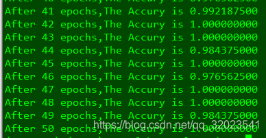
可以看到，使用了栈式自编码预训练后，得到的网络几乎可达到 100% 的准确率，对比之前的 mnist 数据集的 97 % 的准确率有所提升。

自编码网络的使用方法 -- 栈式自编码神经网络 SA

猜你喜欢