一、MNIST数据集读取
one hot 独热编码
独热编码是一种稀疏向量,其中:一个向量设为1,其他元素均设为0.独热编码常用于表示拥有有限个可能值的字符串或标识符
优点: 1、将离散特征的取值扩展到了欧式空间,离散特征的某个取值就对应欧式空间的某个点
2、机器学习算法中,特征之间距离的计算或相似度的常用计算方法都是基于欧式空间的
3、将离散型特征使用one_hot编码,会让特征之间的距离计算更加合理
import tensorflow as tf
 #MNIST数据集读取
import tensorflow.examples.tutorials.mnist.input_data as input_data
mnist = input_data.read_data_sets("MNIST_data/",one_hot=True)

###输出结果###
#若不成功可手动到相关网站下载之后添加到文件夹中
二、了解MNIST手写数字识别数据集
#了解MNIST手写数字识别数据集
print('训练集 train 数量:',mnist.train.num_examples,
      ',验证集 validation 数量:',mnist.validation.num_examples,
      ',测试集 test 数量:',mnist.test.num_examples)

###输出结果###
#训练集 train 数量: 55000 ,验证集 validation 数量: 5000 ,测试集 test 数量: 10000
print(' train images shape:',mnist.train.images.shape,
      'labels shape:',mnist.train.labels.shape)
###输出### #train images shape: (55000, 784) labels shape: (55000, 10)
#28*28=784,10分类One Hot编码
三、可视化image
#可视化image
import matplotlib.pyplot as plt

def plot_image(image):
    plt.imshow(image.reshape(28,28),cmap='binary')
    plt.show()
plot_image(mnist.train.images[1])
输出结果:

#进一步了解reshape()
import numpy as np
int_array = np.array([i for i in range(64)])
print(int_array)
输出结果:
[ 0  1  2  3  4  5  6  7  8  9 10 11 12 13 14 15 16 17 18 19 20 21 22 23 24
 25 26 27 28 29 30 31 32 33 34 35 36 37 38 39 40 41 42 43 44 45 46 47 48 49
 50 51 52 53 54 55 56 57 58 59 60 61 62 63]
int_array.reshape(8,8)
输出结果:
#行优先,逐列排列
int_array.reshape(4,16)
输出结果:
array([[ 0,  1,  2,  3,  4,  5,  6,  7,  8,  9, 10, 11, 12, 13, 14, 15],
       [16, 17, 18, 19, 20, 21, 22, 23, 24, 25, 26, 27, 28, 29, 30, 31],
       [32, 33, 34, 35, 36, 37, 38, 39, 40, 41, 42, 43, 44, 45, 46, 47],
       [48, 49, 50, 51, 52, 53, 54, 55, 56, 57, 58, 59, 60, 61, 62, 63]])
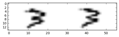
plt.imshow(mnist.train.images[20000].reshape(14,56),cmap='binary')
plt.show()
输出结果:
四、数据读取
1.采用独热编码,标签数据内容并不是直接输出值,而是输出编码
#标签数据与独热编码,
#内容并不是直接输出值,而是输出编码
mnist.train.labels[1]
输出结果:
array([ 0., 0., 0., 1., 0., 0., 0., 0., 0., 0.])
#非one_hot编码的标签值
mnist_no_one_hot = input_data.read_data_sets("MNIST_data/",one_hot=False)
print(mnist_no_one_hot.train.labels[0:10])      #onr_hot = False,直接返回值
输出结果:
Extracting MNIST_data/train-images-idx3-ubyte.gz
Extracting MNIST_data/train-labels-idx1-ubyte.gz
Extracting MNIST_data/t10k-images-idx3-ubyte.gz
Extracting MNIST_data/t10k-labels-idx1-ubyte.gz
[7 3 4 6 1 8 1 0 9 8]
2.读取验证集数据
#读取验证集数据
print('validation images:',mnist.validation.images.shape,'labels:',mnist.validation.labels.shape)
输出:
validation images: (5000, 784) labels: (5000, 10)
3.读取测试机数据
#读取测试机数据
print('tast images:',mnist.test.images.shape,'labels:',mnist.test.labels.shape)
输出结果:
tast images: (10000, 784) labels: (10000, 10)
4.一次批量读取多条数据
#一次批量读取多条数据
batch_image_xs,batch_labels_ys = mnist.train.next_batch(batch_size=10)        #next_batch()实现内部会对数据集先做shuffle
print(mnist.train.labels[0:10])
print("\n")
print(batch_labels_ys)
输出结果:
[[ 0.  0.  0.  1.  0.  0.  0.  0.  0.  0.]
 [ 0.  0.  0.  0.  0.  0.  1.  0.  0.  0.]
 [ 0.  0.  0.  0.  0.  0.  0.  1.  0.  0.]
 [ 0.  0.  0.  0.  0.  0.  0.  1.  0.  0.]
 [ 0.  0.  0.  0.  0.  0.  0.  1.  0.  0.]
 [ 0.  0.  0.  0.  0.  0.  0.  0.  0.  1.]
 [ 0.  0.  0.  0.  1.  0.  0.  0.  0.  0.]
 [ 0.  0.  0.  0.  0.  0.  0.  0.  1.  0.]
 [ 0.  0.  0.  0.  0.  0.  0.  0.  0.  1.]
 [ 0.  0.  0.  0.  0.  0.  0.  0.  0.  1.]]


[[ 0.  0.  0.  0.  0.  0.  1.  0.  0.  0.]
 [ 0.  0.  0.  0.  0.  1.  0.  0.  0.  0.]
 [ 0.  0.  0.  0.  0.  0.  0.  1.  0.  0.]
 [ 0.  1.  0.  0.  0.  0.  0.  0.  0.  0.]
 [ 0.  0.  0.  0.  0.  0.  0.  0.  0.  1.]
 [ 0.  0.  0.  1.  0.  0.  0.  0.  0.  0.]
 [ 0.  1.  0.  0.  0.  0.  0.  0.  0.  0.]
 [ 0.  0.  0.  0.  0.  0.  0.  0.  1.  0.]
 [ 1.  0.  0.  0.  0.  0.  0.  0.  0.  0.]
 [ 0.  0.  0.  0.  0.  0.  0.  1.  0.  0.]]
5.argmax()用法
argmax返回的是最大数的索引
import numpy as np
np.array(mnist.train.labels[1])
np.argmax(mnist.train.labels[1])     #argmax返回的是最大数的索引
#argmax详解
arr1 = np.array([1,3,2,5,7,0])
arr2 = np.array([[1,2,3],[3,2,1],[4,7,2],[8,3,2]])
print("arr1=",arr1)
print("arr2=",arr2)

argmax_1 = tf.argmax(arr1)
argmax_20 = tf.argmax(arr2,0)      #指定第二个参数为0,按第一维(行)的元素取值,即同列的每一行取值   以行为基准,每列取最大值的下标
argmax_21 = tf.argmax(arr2,1)       #指定第二个参数为1,则第二维(列)的元素取值,即同行的每一列取值   以列为基准,每行取最大值的下标
argmax_22 = tf.argmax(arr2,-1)     #指定第二个参数为-1,则第最后维的元素取值

with tf.Session() as sess:
    print(argmax_1.eval())
    print(argmax_20.eval())
    print(argmax_21.eval())
    print(argmax_22.eval())
输出结果:
arr1= [1 3 2 5 7 0]
arr2= [[1 2 3]
 [3 2 1]
 [4 7 2]
 [8 3 2]]
4
[3 2 0]
[2 0 1 0]
[2 0 1 0]
五、可视化
#定义可视化函数
import matplotlib.pyplot as plt
import numpy as np
def plot_images_labels_prediction(images,labels,prediction,index,num=10):  #参数: 图形列表,标签列表,预测值列表,从第index个开始显示,缺省一次显示10幅
    fig = plt.gcf()             #获取当前图表,Get Current Figure
    fig.set_size_inches(10,12)    #1英寸等于2.45cm
    if num > 25 :      #最多显示25个子图
        num = 25
    for i in range(0,num):
        ax = plt.subplot(5,5,i+1)   #获取当前要处理的子图
        ax.imshow(np.reshape(images[index],(28,28)), cmap = 'binary')              #显示第index个图像
        title = "labels="+str(np.argmax(labels[index]))              #构建该图上要显示的title信息
        if len(prediction)>0:
            title += ",predict="+str(prediction[index])

        ax.set_title(title,fontsize=10)    #显示图上的title信息
        ax.set_xticks([])           #不显示坐标轴
        ax.set_yticks([])
        index += 1
    plt.show()
#可视化预测结果
# plot_images_labels_prediction(mnist.test.images,mnist.test.labels,prediction_result,10,10)

plot_images_labels_prediction(mnist.test.images,mnist.test.labels,prediction_result,10,25)
六、评估与应用
#评估模型
#完成训练后,在测试集上评估模型的准确率
accu_test = sess.run(accuracy,feed_dict={x:mnist.test.images,y:mnist.test.labels})
print("Test Accuracy:",accu_test)
#完成训练后,在验证集上评估模型的准确率
accu_validation = sess.run(accuracy,feed_dict={x:mnist.validation.images,y:mnist.validation.labels})
print("Test Accuracy:",accu_validation)
#完成训练后,在训练集上评估模型的准确率
accu_train = sess.run(accuracy,feed_dict={x:mnist.train.images,y:mnist.train.labels})
print("Test Accuracy:",accu_train)
#应用模型
#在建立模型并进行训练后,若认为准确率可以接受,则可以使用此模型进行预测
#由于pred预测结果是one_hot编码格式,所以需要转换成0~9数字
prediction_result = sess.run(tf.argmax(pred,1),feed_dict={x:mnist.test.images})

#查看预测结果中的前10项
prediction_result[0:10]
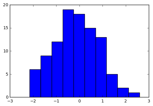
七、tf.random_normal()介绍
#tf.random_normal()介绍
norm = tf.random_normal([100])    #生成100个随机数
with tf.Session() as sess:
    norm_data = norm.eval()
print(norm_data[:10])

import matplotlib.pyplot as plt
plt.hist(norm_data)
plt.show()
输出结果:
[-1.20503342 -0.40912333  1.02314627  0.91239542 -0.44498116  1.46095467
  1.71958613 -0.02297023 -0.04446657 -1.58943892]