大纲:
-数据处理
-模型构建
-拟合效果
1.数据处理
真实业务数据。来源于特步四川分公司。
数据按照地区可以划分为:成都/乐山/南充/绵阳等;按品类可以划分为羽绒服/板鞋/短袖POLO等等。
数据时间跨度:2014年1月~2017年10月
样本:成都地区跑鞋销量预测
#读取数据
library(readxl)
Shoes2_Chengdu <- read_excel("Desktop/跑鞋区域数据.xlsx", sheet = "成都", col_types = c("date", "numeric"))
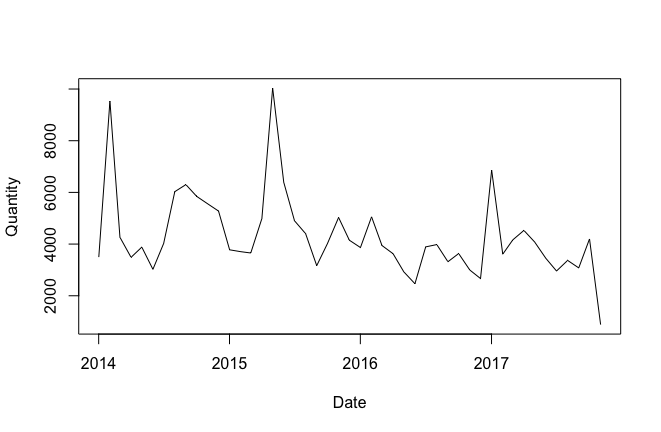
plot(Shoes2_Chengdu,type="line")
attach(Shoes2_Chengdu)
Quantity=as.numeric(Quantity)
detach(Shoes2_Chengdu)绘制趋势图,对整体趋势有一个直观的感受:
节假日因素调整:因为特步在每年的春节,五一,十一等节假日都会举行促销活动。除了春节外,其他的节假日都在固定时间。我们所需要调整的是每年春节的不固定日期。
#调整春节因素,2014年春节在一月
a=Shoes2_Chengdu$Quantity[1]
Shoes2_Chengdu$Quantity[1]=Shoes2_Chengdu$Quantity[2]
Shoes2_Chengdu$Quantity[2]=a
如果有过小的值,代表是反季商品促销。(比如羽绒服在夏季的销量)直接做0值处理,不做预测(因为对销售决策制定没有指导意义)。
#剔除过小的值
for (i in 1:47)
{if(Shoes2_Chengdu$Quantity[i]<20)
  Shoes2_Chengdu$Quantity[i]<-0
}
加载时间序列包,将数据整理成时间序列格式。
#加载时间序列程序包
library(tseries)
library(forecast)
library(dplyr)
library(stats)
#转换成时间序列
Shoes2_Chengduts<-ts(Shoes2_Chengdu$Quantity[1:47],fre=12,start=c(2014,01))通过箱形图检测异常值:箱形图可以用来观察数据整体的分布情况,利用中位数,25/%分位数,75/%分位数,上边界,下边界等统计量来来描述数据的整体分布情况。通过计算这些统计量,生成一个箱体图,箱体包含了大部分的正常数据,而在箱体上边界和下边界之外的,就是异常数据。
(因为样本量跨越年份较少,所以基本检测不出异常值)。如果有异常值,通过插值法调整。#箱型图检测异常值
for(i in 1:12){
bp[,i]<-(Shoes2_Chengduts[c(i,i+12,i+24)])}
bptest=boxplot(bp)
bptest$out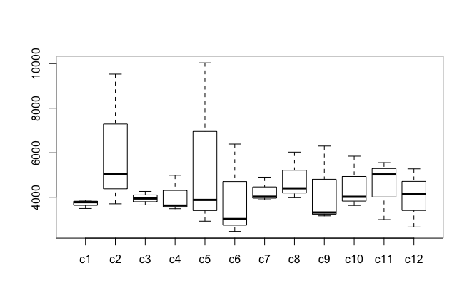
2.模型构建
选择ARIMA模型。
首先先检测模型的平稳性。
#检测一下平稳性
adf.test(Shoes2_Chengduts)
Augmented Dickey-Fuller Test
data: Shoes2_Chengduts
Dickey-Fuller = -7.0728, Lag order = 3, p-value = 0.01
alternative hypothesis: stationary
Warning message:
In adf.test(Shoes2_Chengduts) : p-value smaller than printed p-value可以看出P值很小,我们可以认为模型整体没有向上或向下的趋势,基本平稳。
接下来通过ACF图和PACF图确定模型阶数。
tsdisplay(Shoes2_Chengduts)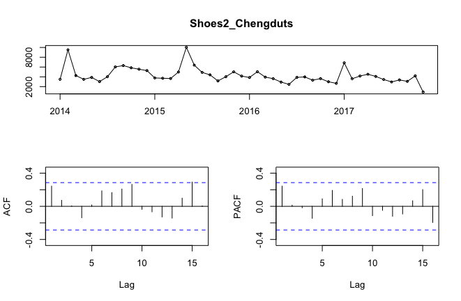
可以看出ACF图并没有明显的截尾的表现,明显存在季节性。实际上我们用常识也可以判断出来,销售每年都是有周期性的。所以我们加入季节性因子,考虑12阶次差分。
adf.test(diff(Shoes2_Chengduts,12)结论同上,平稳。
	Augmented Dickey-Fuller Test

data:  diff(Shoes2_Chengduts, 12)
Dickey-Fuller = -4.005, Lag order = 3, p-value = 0.02093
alternative hypothesis: stationary
做ACF和PACF图
tsdisplay(diff(Shoes2_Chengduts,12))
ACF在1阶处衰减,PACF在1阶处截尾。初步确定Arima阶数为(0,0,0)(1,0,1)[12]
arima1<-arima(Shoes2_Chengduts,order=c(0,0,0),seasonal=list(order=c(2,0,1),period=12))我们再来看一下R中自带的auto命令给出的最优参数。
> auto1<-auto.arima(Shoes2_Chengduts,trace=T)


 ARIMA(2,1,2)(1,0,1)[12] with drift         : Inf
 ARIMA(0,1,0)            with drift         : 830.1212
 ARIMA(1,1,0)(1,0,0)[12] with drift         : 826.1885
 ARIMA(0,1,1)(0,0,1)[12] with drift         : Inf
 ARIMA(0,1,0)                               : 827.9735
 ARIMA(1,1,0)            with drift         : 825.481
 ARIMA(1,1,0)(0,0,1)[12] with drift         : 826.216
 ARIMA(1,1,0)(1,0,1)[12] with drift         : Inf
 ARIMA(2,1,0)            with drift         : 824.9653
 ARIMA(2,1,1)            with drift         : Inf
 ARIMA(3,1,1)            with drift         : Inf
 ARIMA(2,1,0)                               : 822.7944
 ARIMA(2,1,0)(1,0,0)[12]                    : 819.5303
 ARIMA(2,1,0)(1,0,1)[12]                    : 820.9409
 ARIMA(1,1,0)(1,0,0)[12]                    : 824.0301
 ARIMA(3,1,0)(1,0,0)[12]                    : 821.3261
 ARIMA(2,1,1)(1,0,0)[12]                    : 820.4318
 ARIMA(3,1,1)(1,0,0)[12]                    : 820.7753
 ARIMA(2,1,0)(1,0,0)[12] with drift         : 821.4325


 Best model: ARIMA(2,1,0)(1,0,0)[12]
要比较模型的拟合效果,通常使用赤池信息法则(即AIC)来衡量模型的优劣。为了避免过度拟合带来的偏差,AIC中增加了对多余变量的惩罚项。我们可以计算AIC的值,越小的AIC的值说明模型的拟合效果最好。
现在我们需要比较两个模型的AIC值。
arima1$aic
[1] 811.2276
> auto1$aic
[1] 819.5303R函数选择的模型比我们认为比较出来的模型AIC值更高。当然这并不意味着哪个模型“最优”,auto1 的AIC值较高的原因可能是因为加入更多参数,但由于参数值比较大,所以对“过拟合风险”的惩罚项较大。有时候我们需要在衡量过拟合和准确性之间作出抉择。可以最终两者都尝试一下,作出判断。
3.拟合效果
(1)ARIMA1
fit1<-forecast(arima1,h=1,level = c(99.5))plot(fit1)
lines(fit1$fitted,col="green")
lines(Shoes2_Chengduts,col='black')
可以看出在16年之前的拟合曲线有滞后现象。明显感觉有某些因素没考虑到哦。
再来比较2017年的预测精度。
fitvsture<-data.frame(floor(fit1$fitted[37:47]),Shoes2_Chengdu$Quantity[37:47])
#调整春节因素,2017年春节在1月
a<-fitvsture[1,1]
fitvsture[1,1]=fitvsture[2,1]
fitvsture[2,1]=a#精确度校验
d<-Shoes2_Chengdu$Quantity[1:10]
for(i in 1:10){
d[i]<-1-(abs(fitvsture[i,1]-fitvsture[i,2])/max(fitvsture[i,1],fitvsture[i,2]))
}
print(fitvsture)
print(d)
error=sum(d[1:10])/10
print(error)> print(fitvsture)
floor.fit1.fitted.37.47.. Shoes2_Chengduts.37.47.
1 3889 6860
2 3393 3609
3 3935 4162
4 5646 4529
5 4699 4080
6 4724 3453
7 3749 2958
8 3216 3368
9 3281 3078
10 3115 4198
11 3933 883
> print(d[1:10])
[1] 0.5669096 0.9401496 0.9454589 0.8021608 0.8682698 0.7309483 0.7890104
[8] 0.9548694 0.9381286 0.7420200
> error=sum(d[1:10])/10
> print(error)
[1] 0.8277926#11月份数据不足,不做预测。不计入精度排名。预测总精度基本上可以达80%。(2)AUTO1
fit1<-forecast(auto1,h=1,level = c(99.5))
plot(fit1)
lines(fit1$fitted,col="green")
lines(Shoes2_Chengduts,col='black')
fitvsture<-data.frame(floor(fit1$fitted[37:47]),Shoes2_Chengduts[37:47])
#调整春节因素,2017年春节在1月
a<-fitvsture[1,1]
fitvsture[1,1]=fitvsture[2,1]
fitvsture[2,1]=a
fitvsture
#精确度校验
d<-Shoes2_Chengdu$Quantity[1:10]
for(i in 1:10){
d[i]<-1-(abs(fitvsture[i,1]-fitvsture[i,2])/max(fitvsture[i,1],fitvsture[i,2]))
}
print(fitvsture)
print(d[3:10])
error=sum(d[3:10])/7
print(error)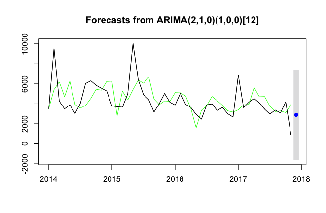
> print(fitvsture)
   floor.fit1.fitted.37.47.. Shoes2_Chengduts.37.47.
1                       3393                    6860
2                       3889                    3609
3                       3935                    4162
4                       5646                    4529
5                       4699                    4080
6                       4724                    3453
7                       3749                    2958
8                       3216                    3368
9                       3281                    3078
10                      3115                    4198
11                      3933                     883
> print(d[1:10])
 [1] 0.4946064 0.9280021 0.9454589 0.8021608 0.8682698 0.7309483 0.7890104
 [8] 0.9548694 0.9381286 0.7420200
> error=sum(d[1:10])/10
> print(error)
[1] 0.8193475
结论:我们可看出,R软件自动生成的模型AUTO1 的整体拟合效果较ARIMA1较差一些,但两者相差很小,精确到小数点后两位后几乎可以忽略不计。为了降低过拟合风险和提高预测精度,我们最终还是选择ARIMA1。