线性回归和梯度下降讲解与代码

本文也是根据吴恩达机器学习课程作业的答案。

回归：预测值是连续的；分类：预测值是离散的；

建模误差：预测值与实际值之间的差距；

目标：选择模型参数，使得建模误差的平方和能够最小，即代价函数最小；

代价函数：选择平方误差函数，是解决回归问题最常用的手段；代价函数是帮助我们选择最优的参数的方法，即设定标准为参数使得建模误差最小；

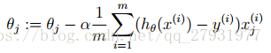
梯度下降：用来求函数最小值的算法，它背后的思想是，开始时随机选择一个参数的组合，计算代价函数，然后寻找下一个能让代价函数值下降最多的参数组合。持续知道得到一个局部最小值。实现梯度下降算法的微妙之处是，同时更新参数；

梯度下降的直观理解：微分部分是那个点的斜率，右边部分的曲线的斜率是不断减小的，局部最优点的斜率为0（假设代价函数为抛物线）；

批量梯度下降：在梯度下降的每一步中，我们都用到了所有的训练样本；

在多变量线性回归中

为了将特征向量化，引入x0=1，故该式实际变量为n。特征矩阵X的维度是m*(n+1)

特征缩放：保证特征都具有相似的尺度（-1,1），将帮助梯度下降算法更快的收敛。

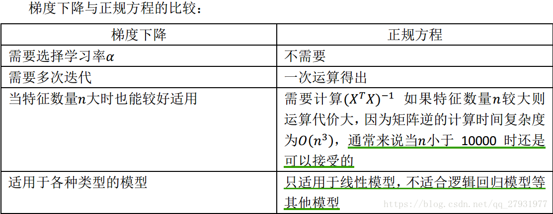
正规方程：求解正规方程找出使得代价函数最小的参数。

线性回归代码实现最主要的部分就是代价函数的计算和梯度下降(对损失函数进行极小化)，即对以下两个公式的实现。在代码最后面专门定义了函数

import matplotlib.pyplot as plt #绘图框架
import numpy as np
from matplotlib.colors import LogNorm #将颜色规范化在log级别的0-1内
from mpl_toolkits.mplot3d import axes3d, Axes3D
from computeCost import *
from gradientDescent import *
from plotData import * #有一个plotData.py的文件需要把代码补齐

# ===================== Part 1: Plotting =====================可视化为了理解数据
print('Plotting Data...')
data = np.loadtxt('ex1data1.txt', delimiter=',', usecols=(0, 1)) #读取文件，分隔值的字符，确定读取的列
X = data[:, 0] #冒号左边是行范围，右边列范围。取二维数组中第一列的所有数据
y = data[:, 1] #取二维数组中第二列的所有数据
m = y.size

plt.ion() #打开交互模式，plt.plot()直接出图像，不需要show()。没有ioff()关闭的话，图像一闪而过，不会常留
plt.figure(0)
plot_data(X, y) #在plotdata.py中定义了一个plot_data的函数

input('Program paused. Press ENTER to continue')

# ===================== Part 2: Gradient descent =====================
print('Running Gradient Descent...')

X = np.c_[np.ones(m), X]  # Add a column of ones to X。np_c按行连接两个矩阵（矩阵左右相加），行数相等
theta = np.zeros(2)  # initialize fitting parameters。 theta = array([0, 0])

# Some gradient descent settings 迭代次数，学习速率（步长）
iterations = 1500 
alpha = 0.01

# Compute and display initial cost
print('Initial cost : ' + str(compute_cost(X, y, theta)) + ' (This value should be about 32.07)') #需要对computerCost.py补全，代价函数=1/2m * sum(f(x)-y)**2)，pdf第五页的公式

theta, J_history = gradient_descent(X, y, theta, alpha, iterations) #在gradientDescent.py处对代码补全

print('Theta found by gradient descent: ' + str(theta.reshape(2)))

# Plot the linear fit
plt.figure(0)
line1, = plt.plot(X[:, 1], np.dot(X, theta), label='Linear Regression')
plt.legend(handles=[line1])

input('Program paused. Press ENTER to continue')

# Predict values for population sizes of 35,000 and 70,000
predict1 = np.dot(np.array([1, 3.5]), theta)
print('For population = 35,000, we predict a profit of {:0.3f} (This value should be about 4519.77)'.format(predict1*10000))
predict2 = np.dot(np.array([1, 7]), theta)
print('For population = 70,000, we predict a profit of {:0.3f} (This value should be about 45342.45)'.format(predict2*10000))

input('Program paused. Press ENTER to continue')

# ===================== Part 3: Visualizing J(theta0, theta1) =====================
print('Visualizing J(theta0, theta1) ...')

theta0_vals = np.linspace(-10, 10, 100) #创建等差数列。起始，终止，样本数
theta1_vals = np.linspace(-1, 4, 100)

xs, ys = np.meshgrid(theta0_vals, theta1_vals) #生成一个坐标矩阵
J_vals = np.zeros(xs.shape)

# Fill out J_vals
for i in range(0, theta0_vals.size):
    for j in range(0, theta1_vals.size):
        t = np.array([theta0_vals[i], theta1_vals[j]])
        J_vals[i][j] = compute_cost(X, y, t)

J_vals = np.transpose(J_vals)

fig1 = plt.figure(1)
ax = fig1.gca(projection='3d')
ax.plot_surface(xs, ys, J_vals)
plt.xlabel(r'$\theta_0$')
plt.ylabel(r'$\theta_1$')

plt.figure(2)
lvls = np.logspace(-2, 3, 20)
plt.contour(xs, ys, J_vals, levels=lvls, norm=LogNorm())
plt.plot(theta[0], theta[1], c='r', marker="x")

input('ex1 Finished. Press ENTER to exit')

def plot_data(x, y):
    plt.scatter(x, y, c = 'r', marker = 'o')
    plt.xlabel('population')
    plt.ylabel('revenue')
    plt.show()

def compute_cost(X, y, theta):
    # Initialize some useful values
    m = y.size
    cost = 0 
    cost = np.sum((np.dot(X, theta) - y)**2) / (2*m)
    return cost

def gradient_descent(X, y, theta, alpha, num_iters):
    # Initialize some useful values
    m = y.size
    J_history = np.zeros(num_iters)

    for i in range(0, num_iters):      
        error = np.dot(X, theta).flatten() - y
        theta -= (alpha/m)*np.sum(X*error[:, np.newaxis], 0)
        
        J_history[i] = compute_cost(X, y, theta)

    return theta, J_history


def gradient_descent_multi(X, y, theta, alpha, num_iters):
    # Initialize some useful values
    m = y.size
    J_history = np.zeros(num_iters)

    for i in range(0, num_iters):
        error = np.dot(X, theta).flatten() - y
        theta -= (alpha / m) * np.sum(X * error[:, np.newaxis], 0)
        J_history[i] = compute_cost(X, y, theta)

    return theta, J_history

线性回归和梯度下降讲解与代码

猜你喜欢