版权声明:本文为博主原创文章,未经博主允许不得转载。 https://blog.csdn.net/qilixuening/article/details/72453632
本题纯粹用作练习,无任何其他意义。
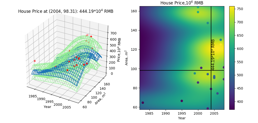
采用高斯基函数作为线性回归模型,用sklearn.gaussian_process.GaussianProcessRegressor可以进行回归,顺便学习画3D图。
代码如下:
# -*- coding: utf-8 -*-
import numpy as np
import matplotlib.pyplot as plt
from sklearn.gaussian_process import GaussianProcessRegressor
from sklearn.gaussian_process.kernels import RBF, ConstantKernel as C
from mpl_toolkits.mplot3d import Axes3D

test = np.array([[2004,98.31]])
data = np.array([
    [2001,100.83,410],[2005,90.9,500],[2007,130.03,550],[2004,78.88,410],[2006,74.22,460],
    [2005,90.4,497],[1983,64.59,370],[2000,164.06,610],[2003,147.5,560],[2003,58.51,408],
    [1999,95.11,565],[2000,85.57,430],[1995,66.44,378],[2003,94.27,498],[2007,125.1,760],
    [2006,111.2,730],[2008,88.99,430],[2005,92.13,506],[2008,101.35,405],[2000,158.9,615]])
kernel = C(0.1, (0.001,0.1))*RBF(0.5,(1e-4,10))
reg = GaussianProcessRegressor(kernel=kernel,n_restarts_optimizer=10,alpha=0.1)
reg.fit(data[:,:-1], data[:,-1])
x_min, x_max = data[:, 0].min() - 1, data[:, 0].max() + 1
y_min, y_max = data[:, 1].min() - 1, data[:, 1].max() + 1
xset, yset = np.meshgrid(np.arange(x_min, x_max, 0.5), np.arange(y_min, y_max, 0.5))
output,err = reg.predict(np.c_[xset.ravel(), yset.ravel()],return_std=True)
output,err = output.reshape(xset.shape),err.reshape(xset.shape)
sigma = np.sum(reg.predict(data[:,:-1], return_std=True)[1])
up,down = output*(1+1.96*err), output*(1-1.96*err)

fig = plt.figure(figsize=(10.5,5))
ax1 = fig.add_subplot(121, projection='3d')
surf = ax1.plot_wireframe(xset,yset,output, rstride=10, cstride=2, antialiased=True)
surf_u = ax1.plot_wireframe(xset,yset,up,colors='lightgreen',linewidths=1,
                            rstride=10, cstride=2, antialiased=True)
surf_d = ax1.plot_wireframe(xset,yset,down,colors='lightgreen',linewidths=1,
                            rstride=10, cstride=2, antialiased=True)
ax1.scatter(data[:,0],data[:,1],data[:,2],c='red')
ax1.set_title('House Price at (2004, 98.31): {0:.2f}$*10^4$ RMB'.format(reg.predict(test)[0]))
ax1.set_xlabel('Year')
ax1.set_ylabel('Area, $m^2$')
ax1.set_zlabel('Price,$10^4$ RMB')

ax = fig.add_subplot(122)
s = ax.scatter(data[:,0],data[:,1],c=data[:,2],cmap=plt.cm.viridis)
# ax.contour(xset,yset,output)
im = ax.imshow(output, interpolation='bilinear', origin='lower',
               extent=(x_min, x_max-1, y_min, y_max), aspect='auto')
plt.colorbar(s,ax=ax)
ax.set_title('House Price,$10^4$ RMB')
ax.hlines(test[0,1],x_min, x_max-1)
ax.vlines(test[0,0],y_min, y_max)
ax.text(test[0,0],test[0,1],'{0:.2f}$*10^4$ RMB'.format(reg.predict(test)[0]),ha='left',va='bottom',color='k',size=11,rotation=90)
ax.set_xlabel('Year')
ax.set_ylabel('Area, $m^2$')
plt.subplots_adjust(left=0.05, top=0.95, right=0.95)
plt.show()