谱图（Spectral Graph Theory）理解（1）

近日看《Semantic Soft Segmentation》（语义软分割），其中一个核心思想是：将来自传统图像处理的底层特征和来自Deep Learning的高级特征，通过谱图（Spectral Graph）框架进行融合，为我们提供了一种机器学习的融合思路和方法。
谱图是图论（Graph Theory）与线性代数（Linear Algebra）的交叉理论，为研究图（Graph）的特性提供了有效方法。本文主要参考【1】，可以认为是它的翻译，但不完全是翻译。

1、预备知识

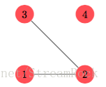
定义1.1：
图（Graph，G）是通过一个顶点（Vertices，V）集合和一个边（Edges，E）集合共同定义的一个对象，而每一边是由一对无序的顶点构成。表示成：
$G=(V,E) \\ E \subseteq V\times V$
我们可以用 $v_i$表示一个顶点，用 $v_{ij}$表示一条连接 $v_i$和 $v_j$的边。本文只讨论 simple graph，即在图中没有Loops（即自己到自己的边），没有 multiple edges（即在两个顶点之间有多条边）。下图是4个顶点 $\{ v_1,v_2,v_3,v_4\}$，两条边 $\{v_{12},v_{23}\}$的 simple graph。

图1
定义1.2：
The order of a graph, $\vert G \vert$, is the size of the set of vertices, $\vert V\vert$.
在这里我将 “order of a graph” 称为图的阶，它就是图中顶点的个数。上图中 $\vert G_1 \vert = 4$。
定义1.3
The degree of a vertex, $\mathbf {deg}(v)$ is the number of edges that are incident with the vertex.
顶点的度（the degree of the vertex）表示从这个顶点发出的edges的数量。对于 $G_1$ 而言， $deg(v_1)=1, deg(v_2)=2, deg(v_3)=1, deg(v_4)=0$。我们称0度的顶点为孤立点（isolated vertex），称1度点为悬垂点（pendant vertex），如图1中， $v_4$ 是孤立点，而 $v_1,v_3$ 是悬垂点。
定义1.4
A walk in a graph is a sequence of alternating vertices and edges that starts and ends at a vertex. A walk of length n is a walk with n edges. Consecutive vertices in the sequence must be connected by an edge in the graph.
Walk——路径（有时也可解释为“游走”、“漫步”），在图中的路径，即从图中一个顶点到另一个顶点，要求这条路径上的前后顶点之间必须有边相连，此walk经过多少条边，则为walk的长度。
定义1.5
A closed walk is a sequence of alternating vertices and edges that starts and ends at the same vertex.
Closed walk——闭环路径，即路径从一个顶点开始，并结束于同一顶点。
定义1.6
A cycle is a closed walk which contains any edge at most one time.
Cycle——环，在闭环路径中，图的任何边都最多只能出现一次。
定义1.7
一个图G被称为连通的（connected），只需要在任意两个顶点之间存在一条长度为k的路径（walk）， $1\le k \le n-1, n=\vert G\vert$
定义1.8
图G的直径（diameter），它等于图中两个顶点最远的距离
我们可以用一幅图画（picture）来描述一个图（graph），圆圈表示顶点，圆圈之间的连线表示边，如图1，另外，我们也可以用一个矩阵来表示graph，它们是等效的，而矩阵的表示方式使我们能通过代数的方法来研究graph，这是两个领域连通的关键。
定义1.9
The adjacency matrix, A, is an nn matrix where n=|G| that represents which vertices are connected by an edge. If vertex i and vertex j are adjacent then $a_{ij}=1$, otherwise $a_{ij}=0$.
adjacency matrix——邻接矩阵，用矩阵的形式表示顶点之间有没有边连接，若G的阶是n，则它是nn矩阵。图1的graph可以表示为：
$\mathbf A = \left[ \begin{array}{cccc} 0&1&0&0\\ 1&0&1&0\\ 0&1&0&0\\ 0&0&0&0 \end{array} \right]$
因为G时simple graph，因此 $a_{ii}=0$，即对角元素为0，这是因为图中 没有Loop。
定理2.1
The entries $a_{ij}$ in $\mathbf A^k$ represent the number of walks of length k from $v_i$ to $v_j$
$\mathbf A^k$表示k个邻接矩阵相乘，其中的元素 $a_{ij}$表示漫步（walk）的步数为k时，两个顶点 $\{v_i, v_j\}$之间路径（起止的顶点是 $\{v_i, v_j\}$）的总条数。即：the $a_{ij}$ entry in $\mathbf A^k$ represent the number of walks of length k between vertices i and j.
如上例：
$\mathbf A^2 = \left[ \begin{array}{cccc} 0&1&0&0\\ 1&0&1&0\\ 0&1&0&0\\ 0&0&0&0 \end{array} \right]\times \left[ \begin{array}{cccc} 0&1&0&0\\ 1&0&1&0\\ 0&1&0&0\\ 0&0&0&0 \end{array} \right]=\left[ \begin{array}{cccc} 1&0&1&0\\ 0&2&0&0\\ 1&0&1&0\\ 0&0&0&0 \end{array} \right]$
$\mathbf A^3 = \left[ \begin{array}{cccc} 1&0&1&0\\ 0&2&0&0\\ 1&0&1&0\\ 0&0&0&0 \end{array} \right]\times \left[ \begin{array}{cccc} 0&1&0&0\\ 1&0&1&0\\ 0&1&0&0\\ 0&0&0&0 \end{array} \right]=\left[ \begin{array}{cccc} 0&2&0&0\\ 2&0&2&0\\ 0&2&0&0\\ 0&0&0&0 \end{array} \right]$
由上定义和定理，可知：一个n阶的全连通（任意两个顶点之间都有walk）图G，其直径必小于等于n-1，其上任意两点之间必有一条walk其长度小于等于n-1。

2、简单图（Simple Graph）的类型

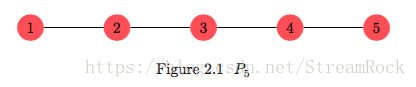
2.1、Path（线型）

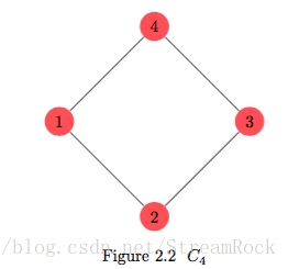
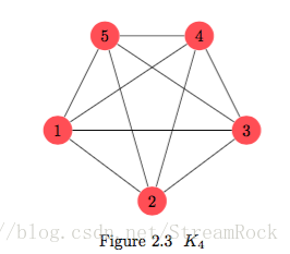
图2 Path型Graph
其邻接矩阵（Adjacency Matrix）为：
$\mathbf A_{Pn}=\left[\begin{array}{ccccccc} 0&1&0&0&\cdots&0&0\\ 1&0&1&0&\cdots&0&0\\ 0&1&0&1&\cdots&0&0\\ 0&0&1&0&\cdots&0&0\\ \vdots&\vdots&\vdots&\vdots&\ddots&\vdots&\vdots\\ 0&0&0&0&\cdots&0&1\\ 0&0&0&0&\cdots&1&0 \end{array} \right]$
2.2、Cycle（环型）

图3 环形Graph
它的Adjacency Matrix比线型的仅有一个差别，就是首尾相连。
$\mathbf A_{Cn}=\left[\begin{array}{ccccccc} 0&1&0&0&\cdots&0&1\\ 1&0&1&0&\cdots&0&0\\ 0&1&0&1&\cdots&0&0\\ 0&0&1&0&\cdots&0&0\\ \vdots&\vdots&\vdots&\vdots&\ddots&\vdots&\vdots\\ 0&0&0&0&\cdots&0&1\\ 1&0&0&0&\cdots&1&0 \end{array} \right]$
2.3、Complete Graph——完全连接图

图4 完全连接
其Adjacency Matrix是：
$\mathbf A_{Kn}=\left[\begin{array}{ccccccc} 0&1&1&1&\cdots&1&1\\ 1&0&1&1&\cdots&1&1\\ 1&1&0&1&\cdots&1&1\\ 1&1&1&0&\cdots&1&1\\ \vdots&\vdots&\vdots&\vdots&\ddots&\vdots&\vdots\\ 1&1&1&1&\cdots&0&1\\ 1&1&1&1&\cdots&1&0 \end{array} \right]$
2.4、Bipartite Graph——二分图
A bipartite graph is a graph on n vertices where the vertices are partitioned into two independent sets, $V_1$ and $V_2$ such that there are no edges between vertices in the same set.
即顶点可分为两个集合： $V_1$ and $V_2$，同一集合中的顶点之间没有边，而不同集合的顶点之间可以有边，如图5。这其实就是两层神经网络节点之间的图的关系：

图5 二分图
其邻接矩阵是：
$\mathbf A = \left[ \begin{array}{cc} \mathbf O & \mathbf B\\ \mathbf B^T & \mathbf O \end{array} \right]$

3、Laplacian Matrix——拉普拉斯矩阵

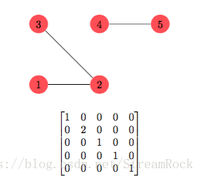
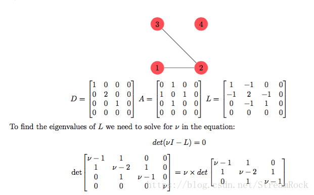
定义3.1
The degree matrix, D, of a graph, G, is the diagonal matrix $D = diag(d_1, d_2, \cdots,d_n)$, where $d_i$ is the degree of vertex i.
度矩阵D，是由各顶点的度（degree）为对角元素所构成的对角矩阵。如：

图6 G的度矩阵（degree matrix）
定义3.2
For a simple graph, G, the laplacian matrix, L=D-A, where D is the degree matrix and A is the adjacency matrix.
关键的一个定义：Laplacian matrix, L=D-A。
Laplacian matrix是一个实对称矩阵（n*n），其特征值（eigenvalue）必大于等于零，表示为 $\{v_1,v_2,\cdots,v_n \}$，共n个，并按顺序排列，即： $v_i \ge v_j, \text{for } \forall i\ge j$。
定义3.3
The trace of a matrix is the sum of the entries along the main diagonal.
方阵的迹。
因而，对于邻接矩阵 $trace(\mathbf A) = \sum_{i=1}^n \lambda_i=0$，对于Laplacian矩阵 $trace(\mathbf L)=\sum_{i=1}^n v_i=\sum_{i=1}^n d_i=2\cdot e(G)$，即Laplacian矩阵的迹是G的边的数量e(G)的2倍。
矩阵L，A，D 的关系举例如下：

可解得L的特征值是 $\{v_1,v_2,v_3,v_4\}=\{3,1,0,0\}$，而adjacency matrix的特征值是 $\{\lambda_1,\lambda_2,\lambda_3,\lambda_4\}=\{\sqrt 2,0,0,-\sqrt 2\}$。所谓的spectrum of a graph指的就是图所对应的Laplacian Matrix的特征值。即 $\{v_1,v_2,v_3,v_4\}=\{3,1,0,0\}$就是上图的谱。
Laplacian Matrix（矩阵L）具有如下性质：
1、 $x^TLx=\frac{1}{2} \sum_{i,j=1}^nw_{ij}(x_i-x_j)^2\text{ for }\forall x \in R^n$
2、 $L\ge0$ if $w_{ij}\ge 0$ for all i,j
3、 $L\cdot\mathbf 1=\mathbf 0$
4、If the underlying graph of G is connected, then
$0=\lambda_1<\lambda_2\le\lambda_3\cdots\le\lambda_n$
5、If the underlying graph of G is connected, then the dimension of the nullspace of L is 1.
对矩阵 $\mathbf L$ 归一化，有：
$\mathcal L=\mathbf D^{-\frac{1}{2}}\mathbf L\mathbf D^{-\frac{1}{2}}=\mathbf D^{-\frac{1}{2}}(\mathbf D - \mathbf A)\mathbf D^{-\frac{1}{2}}=\mathbf I-\mathbf S$
于是归一化Laplacian的元素为：
$\mathcal L(i,j)= \begin{cases} 1, & \text{if $u=v$ and $d_v\neq 0$} \\ -\frac{1}{\sqrt{d_ud_v}}, & \text{if $u$ and $v$ are adjacent}\\ 0, & \text{otherwise} \end{cases}$
谱反映了图的特性，可作为图的结构的研究方法。

---

本文主要是参考【1】，因其内容较基础和简单。
参考文献
1、《Spectral of Simple Graphs》Owen Jones, Whitman College,
May 13, 2013
2、《Sprectral Graph Theory》Fan R. K. Chung