版权声明:本文为博主原创文章,未经博主允许欢迎转载,但请注明出处。 https://blog.csdn.net/liumiaocn/article/details/82916787
活用可视化的结果,使用真正的人类智能,可以一目了然的了解的算法过程中的大致过程,这就是可视化可以带来的结果,在机器学习结果的展示上,能画出来的就尽量不要以数字的形式print出来,这篇文章继续分析y=3*x + 1的收敛过程,这里我们来使用图形化的方式来体验tensorflow的强大。

事前准备
关于线性回归的详细,请参看:
代码准备
代码说明部分也参看如下文章:
过程确认:100次迭代,每十次确认一下拟合状态,代码如下
for j in range(100):
  for i in range(100):
    sess.run(trainoperation, feed_dict={X: xdata[i], Y:ydata[i]})
  if j % 10 == 0:
    print("j = %s index = %s" %(j,index))
    plt.subplot(2,5,index)
    plt.scatter(xdata,ydata)
    labelinfo="iteration: " + str(j)
    plt.plot(xdata,B.eval(session=sess)+W.eval(session=sess)*xdata,'b',label=labelinfo)
    plt.plot(xdata,ydata,'r',label='expected')
    plt.legend()
    index = index + 1
示例代码
liumiaocn:Notebook liumiao$ cat basic-operation-8.py
import tensorflow as tf
import numpy      as np
import os
import matplotlib.pyplot as plt

os.environ['TF_CPP_MIN_LOG_LEVEL'] = '2'

xdata = np.linspace(0,1,100)
ydata = 2 * xdata + 1

print("init modole ...")
X = tf.placeholder("float",name="X")
Y = tf.placeholder("float",name="Y")
W = tf.Variable(3., name="W")
B = tf.Variable(3., name="B")
linearmodel = tf.add(tf.multiply(X,W),B)
lossfunc = (tf.pow(Y - linearmodel, 2))
learningrate = 0.01

print("set Optimizer")
trainoperation = tf.train.GradientDescentOptimizer(learningrate).minimize(lossfunc)

sess = tf.Session()
init = tf.global_variables_initializer()
sess.run(init)

index = 1
print("caculation begins ...")
for j in range(100):
  for i in range(100):
    sess.run(trainoperation, feed_dict={X: xdata[i], Y:ydata[i]})
  if j % 10 == 0:
    print("j = %s index = %s" %(j,index))
    plt.subplot(2,5,index)
    plt.scatter(xdata,ydata)
    labelinfo="iteration: " + str(j)
    plt.plot(xdata,B.eval(session=sess)+W.eval(session=sess)*xdata,'b',label=labelinfo)
    plt.plot(xdata,ydata,'r',label='expected')
    plt.legend()
    index = index + 1

print("caculation ends ...")
print("##After Caculation: ")
print("   B: " + str(B.eval(session=sess)) + ", W : " + str(W.eval(session=sess)))

plt.show()
liumiaocn:Notebook liumiao$
结果确认
从结果可以看到,第一个10次的迭代完成之后就已经非常好的收敛了
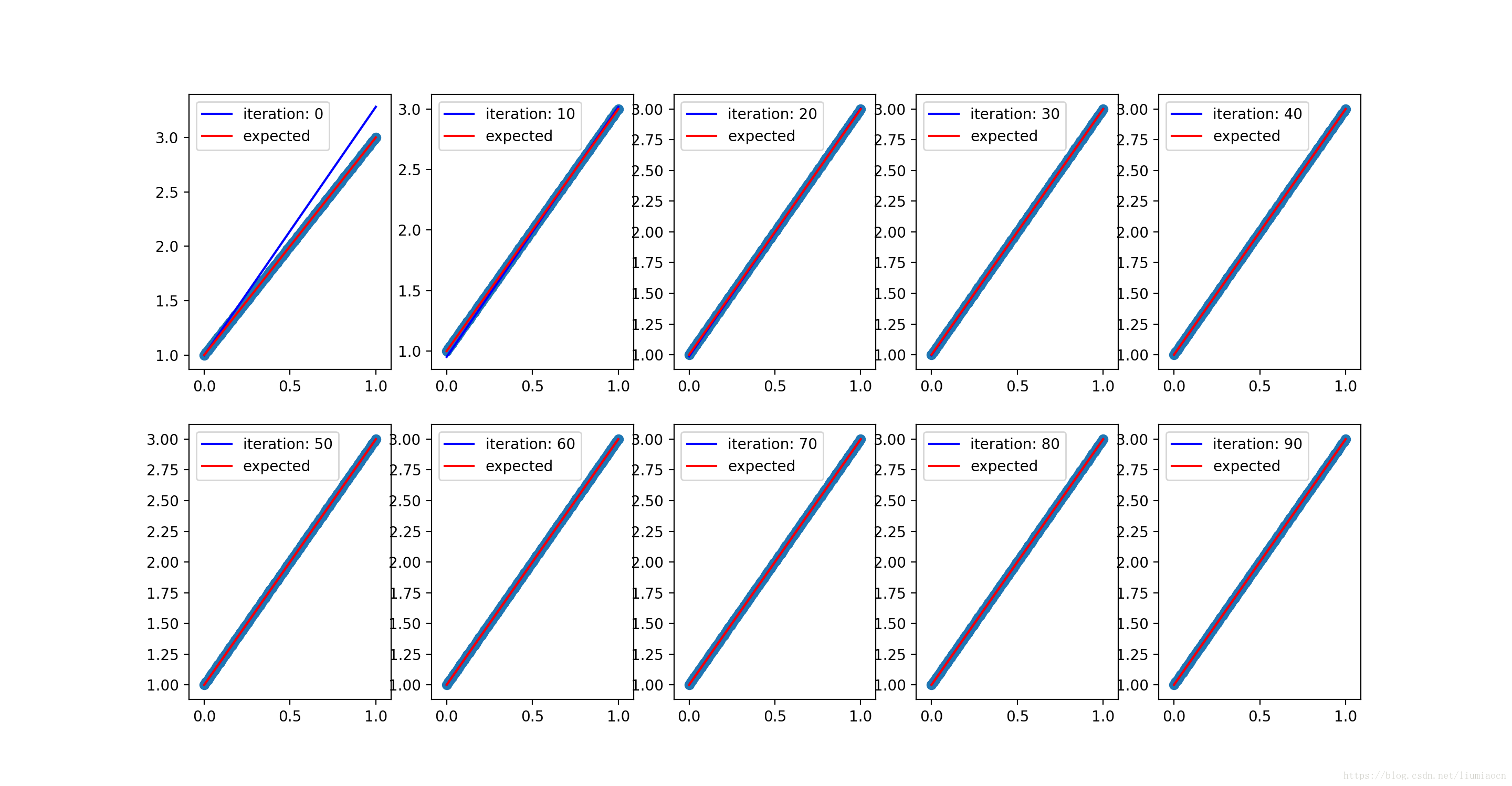
这样,我们调整一下迭代的次数:从100 改为10
for j in range(10):
  for i in range(100):
    sess.run(trainoperation, feed_dict={X: xdata[i], Y:ydata[i]})
  print("j = %s index = %s" %(j,index))
  plt.subplot(2,5,index)
  plt.scatter(xdata,ydata)
  labelinfo="iteration: " + str(j)
  plt.plot(xdata,B.eval(session=sess)+W.eval(session=sess)*xdata,'b',label=labelinfo)
  plt.plot(xdata,ydata,'r',label='expected')
  plt.legend()
  index = index + 1
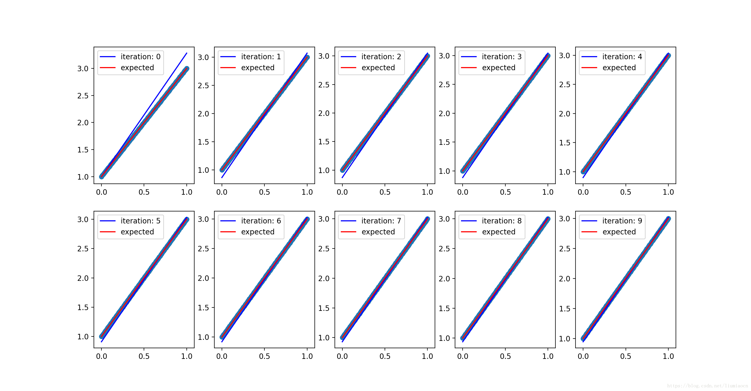
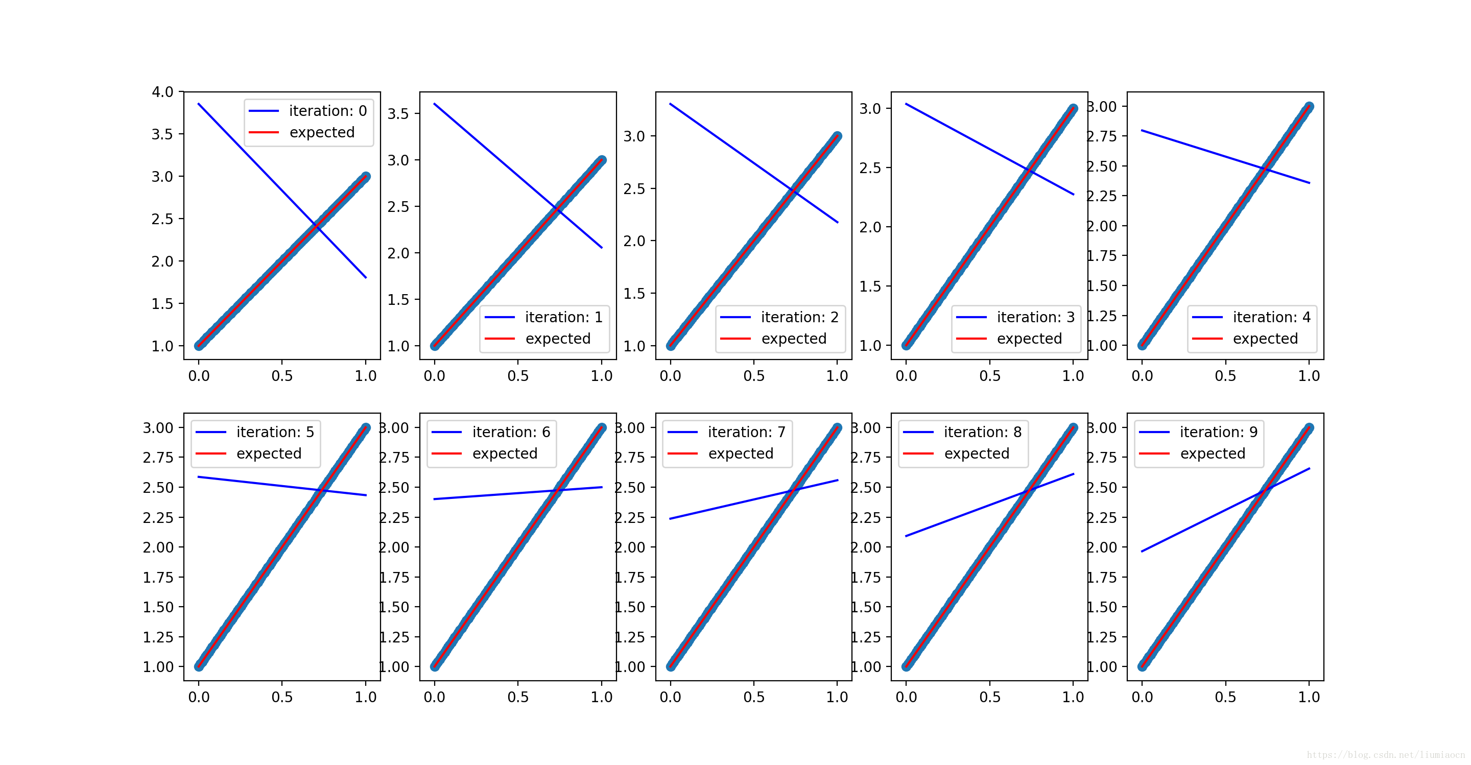
发现依然训练逼近的过程不是很清晰,从最开始都非常清楚,仔细确认一下初始值,W的期待值是3,初始值是2,从最开始就比较准确,所以来调整一下,变成-3,再用同样的代码确认一下
可以清晰地看出调整的过程已经开始逐步逼近了,W为-3的初始值的情况下,每10次迭代粒度来确认一下训练拟合的过程:
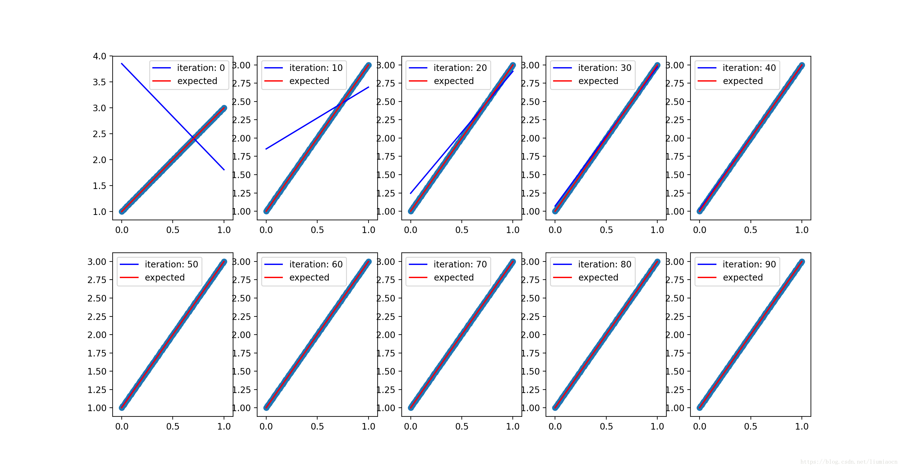
总结
通过对训练过程的可视化结果确认,发现训练的过程会受很多因素的影响,但是总体来说还是能够收敛。tensorflow提供的函数非常强大,很多都像是积木一样方便,通过设定诸如LearningRate这样的值,灵活结合这些图形可视化的库函数,对于初期的学习能起到很好的辅助作用。