版权声明:站在巨人的肩膀上学习。 https://blog.csdn.net/zgcr654321/article/details/84146576
搭建第一个RNN-LSTM神经网络(回归):
我们使用sin函数的y值作为输入数据,然后预测cos函数的y值作为输出数据。
先建立一组等差数列的数组,都除以π作为弧度值,然后分别计算其sin值(作为输入的x数据)和cos值(作为输出的真实值)。
定义一个RNN——LSTM网络结构,包括一个输入层、一个cell层、一个输出层,定义损失函数为方差函数,优化器使用Adam算法。
迭代训练1000次,每50次打印一次batch_size个样本的平均loss值。
代码如下:
import tensorflow as tf
import matplotlib.pyplot as plt
import numpy as np
import os

os.environ['TF_CPP_MIN_LOG_LEVEL'] = '2'
os.environ["CUDA_VISIBLE_DEVICES"] = "0"

# 使用到自己创建的sin值作为输入数据预测一条cos曲线(输出数据)
# 建立train_batch_size样本时候的起始index
batch_index_start = 0
# 时间步数
time_steps = 20
# 每个时间步取的训练样本数量
train_batch_size = 50
# 每个time_steps内输入的数据量
input_size = 1
# 每个time_steps内输出的数据量
output_size = 1
# RNN的hidden_unit的数量
cell_size = 10
# 学习速率
lr = 0.006
# 迭代训练次数
iteration = 1000


def get_next_batch(tm_steps):
	global batch_index_start
	# 一共tm_steps * train_batch_size个样本,xs的shape变为(train_batch_size, tm_steps),并且全部除以π,化为弧度值,即为输入的x数据
	# 每次生成batch_size个样本,每个样本就是一个time_steps中输入的数据量,定为20
	xs = np.arange(batch_index_start, batch_index_start + tm_steps * train_batch_size).reshape(
		(train_batch_size, tm_steps)) / (10 * np.pi)
	# 返回弧度的正弦值,即输入的x数据
	seq = np.sin(xs)
	# 返回弧度的余弦值,即输入的y数据
	# 我们的任务是用输入的x正弦值去预测弧度的余弦值,为了比对,我们预先计算出真实的弧度对应的余弦值
	res = np.cos(xs)
	# 每生成一次样本后,下一次样本开始的index直接从上一次生成的样本末尾的index之后开始
	batch_index_start += tm_steps
	# returned seq, res and xs: shape (batch, step, input)
	return seq[:, :, None], res[:, :, None], xs


# 一个定义LSTM网络结构,含创建输入层、创建隐藏层、创建输出层、计算cost函数等方法的类
class LstmRnn(object):
	def __init__(self, n_steps, ipt_size, opt_size, cl_size, bt_size):
		"""
		:param n_steps: 输入数据的时间步数
		:param ipt_size: 每个时间步中输入数据的数据量
		:param opt_size: 每个时间步中输出数据的数据量
		:param cl_size: 隐藏层神经单元数量
		:param bt_size: 一次迭代训练的样本数量
		"""
		self.n_steps = n_steps
		self.input_size = ipt_size
		self.output_size = opt_size
		self.cell_size = cl_size
		self.batch_size = bt_size
		# 定义X和Y占位符
		with tf.name_scope('inputs'):
			self.X = tf.placeholder(tf.float32, [None, n_steps, ipt_size], name='xs')
			self.Y = tf.placeholder(tf.float32, [None, n_steps, opt_size], name='ys')
		# 定义输入层
		with tf.variable_scope('input_layer'):
			self.add_input_layer()
		# 定义隐藏层也就是cell层
		with tf.variable_scope('LSTM_cell'):
			self.add_cell()
		# 定义输出层
		with tf.variable_scope('output_layer'):
			self.add_output_layer()
		# 定义cost函数
		with tf.name_scope('cost'):
			self.compute_cost()
		# 定义优化器,采用Adam算法
		with tf.name_scope('train'):
			self.train_op = tf.train.AdamOptimizer(lr).minimize(self.cost)

	# 添加输入层的函数
	def add_input_layer(self, ):
		# 输入数据先reshape成(batch*n_step, input_size)
		x_in = tf.reshape(self.X, [-1, self.input_size], name='2_2D')
		# W权重矩阵shape=(input_size, cell_size)
		w_in = self.weight_variable([self.input_size, self.cell_size])
		# b权重矩阵shape=(cell_size, )
		b_in = self.bias_variable([self.cell_size, ])
		# y_in_out的shape = (batch*n_steps, cell_size)
		with tf.name_scope('Wx_plus_b'):
			y_in_out = tf.matmul(x_in, w_in) + b_in
		# reshape y_in_out,其shape=(batch, n_steps, cell_size),这是三维时的形式
		self.y_in_out = tf.reshape(y_in_out, [-1, self.n_steps, self.cell_size], name='2_3D')

	# 添加cell层(隐藏层)
	def add_cell(self):
		# tf.nn.rnn_cell.BasicLSTMCell(n_hidden, forget_bias=1.0, state_is_tuple=True):
		# self.cell_size表示cell层中神经元的个数,forget_bias就是LSTM们的忘记系数,如果等于1,就是不会忘记任何信息。如果等于0,就都忘记。
		# state_is_tuple默认就是True,官方建议用True,就是表示返回的状态用一个元组表示。
		lstm_cell = tf.contrib.rnn.BasicLSTMCell(self.cell_size, forget_bias=1.0, state_is_tuple=True)
		with tf.name_scope('initial_state'):
			# 状态初始化函数zero_state(batch_size,dtype):batch_size就是输入样本批次的数目,dtype就是数据类型,state初始化为全零
			# time_major如果是True,就表示RNN的steps用第一个维度表示,如果是False,那么输入的第二个维度就是steps。
			# 为True时,我们是以LSTM为tf.nn.dynamic_rnn的输入cell类型,此时state形状为[2,batch_size, cell.output_size];
			# 为False时,以GRU为tf.nn.dynamic_rnn的输入cell类型,此时state形状为[batch_size, cell.output_size]。
			self.cell_init_state = lstm_cell.zero_state(self.batch_size, dtype=tf.float32)
			# 如果cell选择了LSTM,那final_state是个tuple,分别代表Ct和ht,其中ht与outputs中的对应的最后一个时刻的输出相等;
			# c和h的维度都是[batch_size, n_hidden]
			# 假设final_state形状为[2,batch_size, cell.output_size],outputs形状为[batch_size, max_time, cell.output_size]
			# 那么final_state[1,batch_size,:] == outputs[batch_size, -1,:]
			# 如果cell是GRU,final_state其实就是ht,final_state==outputs[-1]
			# 其原因是因为LSTM和GRU的结构本身不同
			# 当cell为GRU时,state就只有一个了,原因是GRU将Ct和ht进行了简化,将其合并成了ht
			# GRU将遗忘门和输入门合并成了更新门,另外cell不在有细胞状态cell state,只有hidden state。
			# output里面,包含了所有时刻的输出h
			# state里面,包含了最后一个时刻的输出Ct和ht
			# 如果只需要最后一个时刻的状态输出,直接使用cell_final_state里面的ht输出就可以了。即final_state[1]
			self.cell_outputs, self.cell_final_state = tf.nn.dynamic_rnn(lstm_cell, self.y_in_out,
																		 initial_state=self.cell_init_state,
																		 time_major=False)

	# 建立输出层的函数
	def add_output_layer(self):
		# 输入数据的shape = (batch * steps, cell_size)
		x_out_in = tf.reshape(self.cell_outputs, [-1, self.cell_size], name='2_2D')
		w_out = self.weight_variable([self.cell_size, self.output_size])
		b_out = self.bias_variable([self.output_size, ])
		# 预测出的值的shape = (batch * steps, output_size)
		with tf.name_scope('Wx_plus_b'):
			self.pred = tf.matmul(x_out_in, w_out) + b_out

	# 定义损失函数
	def compute_cost(self):
		# 将上面输出层的输出数据使用sequence_loss_by_example()函数计算,这个函数在内部默认调用的是sparse_softmax_cross_entropy_with_logits()函数
		# 但是我们在下面将损失函数改成了方差函数
		# 也就是计算输出值经过loss函数处理后的加权平均损失,这里的平均是对所有时间序列的输出数据的平均
		# pred传入的list的应该是n_step个二维数组,每个二维数组应该是batch_size * output_size,target和weight参数也是同理。
		# 第一个参数是pred的标签,第二个参数是真实标签,第三个参数就是我们的加权,这里全部设为1,就是正常的平均损失,这里的平均是对所有时间序列的输出数据的平均
		# sequence_loss_by_example(logits, targets, weights,average_across_timesteps=True,softmax_loss_function=None,
		# name=None)
		losses = tf.contrib.legacy_seq2seq.sequence_loss_by_example(
			[tf.reshape(self.pred, [-1], name='reshape_pred')],
			[tf.reshape(self.Y, [-1], name='reshape_target')],
			[tf.ones([self.batch_size * self.n_steps], dtype=tf.float32)],
			average_across_timesteps=True,
			# 这里即将默认的sotfmax_loss_function损失函数改为我们自己定义的方差函数
			softmax_loss_function=self.ms_error,
			name='losses'
		)
		# 计算对一个batch_size样本的平均交叉熵损失
		with tf.name_scope('average_cost'):
			self.cost = tf.div(tf.reduce_sum(losses, name='losses_sum'), self.batch_size, name='average_cost')
			tf.summary.scalar('cost', self.cost)

	def ms_error(self, labels, logits):
		# 注意第2和第3个参数必须要用labels和logits这两个名字!!!
		# 换了别的名字比如y_pred之类的就会报错:TypeError: ms_error() got an unexpected keyword argument 'labels'
		# 大概是因为sequence_loss_by_example()函数中的参数softmax_loss_function接受的真实标签和预测标签必须要用这两个专有的名字labels和logits吧
		return tf.square(tf.subtract(labels, logits))

	# 生成W权重的函数
	def weight_variable(self, shape, name='weights'):
		initializer = tf.random_normal_initializer(mean=0., stddev=1., )
		return tf.get_variable(shape=shape, initializer=initializer, name=name)

	# 生成b权重的函数
	def bias_variable(self, shape, name='biases'):
		initializer = tf.constant_initializer(0.1)
		return tf.get_variable(name=name, shape=shape, initializer=initializer)


if __name__ == '__main__':
	LSTM_model = LstmRnn(time_steps, input_size, output_size, cell_size, train_batch_size)
	with tf.Session() as sess:
		sess.run(tf.global_variables_initializer())
		# 迭代训练iteration次
		for i in range(iteration):
			# 生成一个训练样本
			seq_sin_x, res_cos_y, rad = get_next_batch(time_steps)
			if i == 0:
				# 初始化要喂给模型的数据
				feed_dict = {LSTM_model.X: seq_sin_x, LSTM_model.Y: res_cos_y, }
			else:
				# 如果不是第一次迭代训练,则使用上一次训练的最后一个时刻的state数据作为下一次训练的state数据的初始值
				feed_dict = {LSTM_model.X: seq_sin_x, LSTM_model.Y: res_cos_y, LSTM_model.cell_init_state: state}
			_, cost, state, pred = sess.run(
				[LSTM_model.train_op, LSTM_model.cost, LSTM_model.cell_final_state, LSTM_model.pred],
				feed_dict=feed_dict)
			# 每迭代训练20次,打印一次cost值
			if i % 50 == 0:
				print("iteration:{} cost:{}".format(i, cost))
运行结果如下:
iteration:0 cost:17.073490142822266
iteration:50 cost:2.875434160232544
iteration:100 cost:0.5915642380714417
iteration:150 cost:0.07965247333049774
iteration:200 cost:0.09998466819524765
iteration:250 cost:0.017578929662704468
iteration:300 cost:0.08757047355175018
iteration:350 cost:0.14417988061904907
iteration:400 cost:0.12553825974464417
iteration:450 cost:0.07623404264450073
iteration:500 cost:0.004498453810811043
iteration:550 cost:0.10774078220129013
iteration:600 cost:0.01944294013082981
iteration:650 cost:0.11099396646022797
iteration:700 cost:0.024452701210975647
iteration:750 cost:0.00637128995731473
iteration:800 cost:0.014249494299292564
iteration:850 cost:0.030684275552630424
iteration:900 cost:0.0163046196103096
iteration:950 cost:0.009187780320644379

Process finished with exit code 0
训练过程的matplotlib可视化:
在上面定义代码的模型时,我们已经有意识地将各个部分定义在了各自的命名空间之下。我们可以使用tensorboard工具添加几行简单的代码即可显示出这个模型的结构,这里不再赘述。
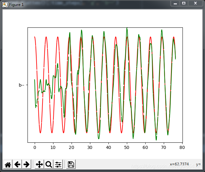
下面我们使用matplotlib可视化我们训练过程中的输出值,看看我们的模型每轮预测的值与真实值的对比,在一个会动态更新的matplotlib图上显示出来。
把上面的代码中的if __name__ == '__main__':这行及以下所有行的代码修改为:
if __name__ == '__main__':
	LSTM_model = LstmRnn(time_steps, input_size, output_size, cell_size, train_batch_size)
	with tf.Session() as sess:
		sess.run(tf.global_variables_initializer())
		# 迭代训练iteration次
		for i in range(iteration):
			# 生成一个训练样本
			seq_sin_x, res_cos_y, rad = get_next_batch(time_steps)
			if i == 0:
				# 初始化要喂给模型的数据
				feed_dict = {LSTM_model.X: seq_sin_x, LSTM_model.Y: res_cos_y, }
			else:
				# 如果不是第一次迭代训练,则使用上一次训练的最后一个时刻的state数据作为下一次训练的state数据的初始值
				feed_dict = {LSTM_model.X: seq_sin_x, LSTM_model.Y: res_cos_y, LSTM_model.cell_init_state: state}
			# 设定一个连续的plot图
			plt.ion()
			# 显示该图
			plt.show()
			_, cost, state, pred = sess.run(
				[LSTM_model.train_op, LSTM_model.cost, LSTM_model.cell_final_state, LSTM_model.pred],
				feed_dict=feed_dict)
			# 画新的曲线段
			# rad[0, :]提取rad第0维上的第0个元素,即第一行的所有rad值,一共20个
			# res_cos_y的shape=(batch, step, input),是个三维数组
			# res_cos_y[0].flatten()提取cos_y的第0个维度上的第0号元素,即第0号样本的全部y数据,一共20个
			#  pred.flatten()[:time_steps]也提取了pred预测的20个y数据
			# 把它们两个都画成曲线段在图上显示出来
			# 需要注意的是,我们实际每次迭代使用了50个样本,但是在图上每次迭代时只画了第0号样本的x和y_true、x和y_pred的曲线
			# 当然你也可以选择将50个样本的数据都画出来,因为我们取得一个batch_size样本时,rad的值是按行排列等差递增的
			plt.plot(rad[0, :], res_cos_y[0].flatten(), 'r', rad[0, :], pred.flatten()[:time_steps], 'g', 'b--')
			# 设定显示出的y轴的最大值和最小值范围
			plt.ylim((-1.2, 1.2))
			# 将上面的新点画在plot图上
			plt.draw()
			# 每画一次停顿0.2s
			plt.pause(0.2)
			# 每迭代训练20次,打印一次cost值
			if i % 20 == 0:
				print("iteration:{} cost:{}".format(i, cost))
运行结果如下:
这里我并没有将1000次迭代运行完。
iteration:0 cost:15.108439445495605
iteration:20 cost:6.4789862632751465
iteration:40 cost:1.2082581520080566
iteration:60 cost:0.6827635169029236
iteration:80 cost:1.5816880464553833
iteration:100 cost:0.4396807849407196
此时这个图会随着我们的迭代不断更新。