TensorFlow入门教程之7：Tensorboard可视化

人工智能/机器学习/深度学习交流QQ群：964753462 也可以扫一扫下面二维码加入微信群，如果二维码失效，可以添加博主个人微信，拉你进群微信公众号：分享人工智能最新技术、职业发展以及个人成长

这篇博客将介绍tensorflow当中一个非常有用的可视化工具tensorboard的使用，它将对我们分析训练效果，理解训练框架和优化算法有很大的帮助。

1. 实验1-矩阵相乘

import tensorflow as tf

with tf.name_scope('graph') as scope:
     matrix1 = tf.constant([[3., 3.]],name ='matrix1')  #1 row by 2 column
     matrix2 = tf.constant([[2.],[2.]],name ='matrix2') # 2 row by 1 column
     product = tf.matmul(matrix1, matrix2,name='product')
  
sess = tf.Session()

writer = tf.summary.FileWriter("logs/", sess.graph)

init = tf.global_variables_initializer()

sess.run(init)

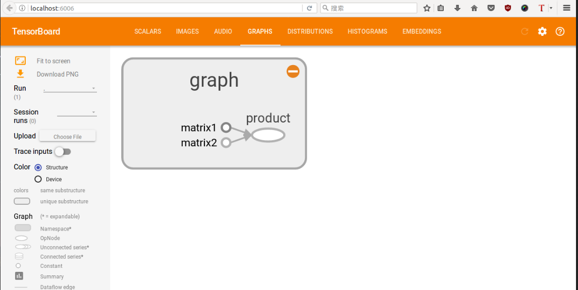
这里相对于第一篇tensorflow多了一点东西，tf.name_scope函数是作用域名，上述代码斯即在graph作用域op下，又有三个op（分别是matrix1，matrix2，product),用tf函数内部的name参数命名，这样会在tensorboard中显示，具体图像还请看下面。

很重要： 运行上面的代码，查询当前目录，就可以找到一个新生成的文件，已命名为logs，然后运行tensorboard --logdir logs指令，然后在浏览器中打开链接：http://localhost:6006 ，如果出现下图，则证明打开成功。
在这里插入图片描述

2. 实验2-线性拟合

2.1 实验2.1

上面那一个是小试牛刀，比较简单，没有任何训练过程。下面用个线性拟合的例子来说明训练过程的可视化。

import tensorflow as tf
import numpy as np

## prepare the original data
with tf.name_scope('data'):
     x_data = np.random.rand(100).astype(np.float32)
     y_data = 0.3*x_data+0.1
##creat parameters
with tf.name_scope('parameters'):
     weight = tf.Variable(tf.random_uniform([1],-1.0,1.0))
     bias = tf.Variable(tf.zeros([1]))
##get y_prediction
with tf.name_scope('y_prediction'):
     y_prediction = weight*x_data+bias
##compute the loss
with tf.name_scope('loss'):
     loss = tf.reduce_mean(tf.square(y_data-y_prediction))
##creat optimizer
optimizer = tf.train.GradientDescentOptimizer(0.5)
#creat train ,minimize the loss 
with tf.name_scope('train'):
     train = optimizer.minimize(loss)
#creat init
with tf.name_scope('init'): 
     init = tf.global_variables_initializer()
##creat a Session 
sess = tf.Session()
##initialize
writer = tf.summary.FileWriter("logs/", sess.graph)
sess.run(init)
## Loop
for step  in  range(101):
    sess.run(train)
    if step %10==0 :
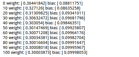
        print step ,'weight:',sess.run(weight),'bias:',sess.run(bias)

运行这个程序会打印一些东西，具体输出如下：
在这里插入图片描述
运行如下Tensorboard命令：

tensorboard --logdir logs/

打开链接，会出现下图：
在这里插入图片描述
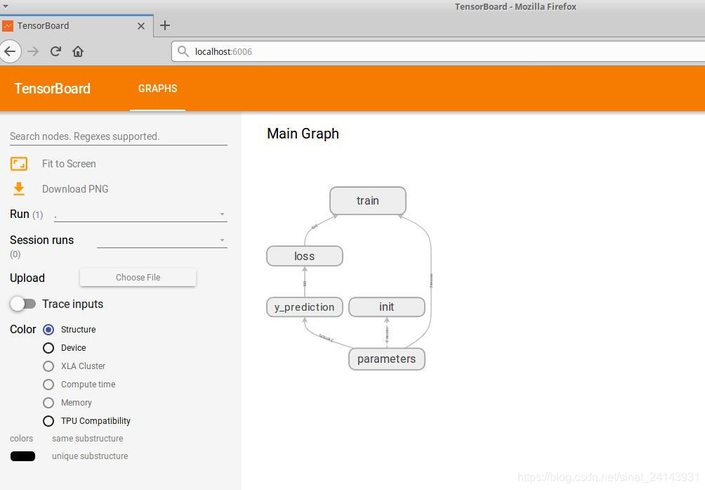
这个就是上面代码的流动图，先初始化参数，算出预测，计算损失，然后训练，更新相应的参数。

当然这个图还可以进行展开，里面有更详细的流动(截图无法全面，还请自己运行出看看哦)

2.2 实验2.2

我们在对上面的代码进行再修改修改，试试tensorboard的其他功能，例如scalars，distributions，histograms,它们对我们分析学习算法的性能有很大帮助。
代码如下：

import tensorflow as tf
import numpy as np

## prepare the original data
with tf.name_scope('data'):
     x_data = np.random.rand(100).astype(np.float32)
     y_data = 0.3*x_data+0.1
##creat parameters
with tf.name_scope('parameters'):
     with tf.name_scope('weights'):
            weight = tf.Variable(tf.random_uniform([1],-1.0,1.0))
           tf.summary.histogram('weight',weight)
     with tf.name_scope('biases'):
           bias = tf.Variable(tf.zeros([1]))
           tf.summary.histogram('bias',bias)
##get y_prediction
with tf.name_scope('y_prediction'):
     y_prediction = weight*x_data+bias
##compute the loss
with tf.name_scope('loss'):
     loss = tf.reduce_mean(tf.square(y_data-y_prediction))
     tf.summary.scalar('loss',loss)
##creat optimizer
optimizer = tf.train.GradientDescentOptimizer(0.5)
#creat train ,minimize the loss 
with tf.name_scope('train'):
     train = optimizer.minimize(loss)
#creat init
with tf.name_scope('init'): 
     init = tf.global_variables_initializer()
##creat a Session 
sess = tf.Session()
#merged
merged = tf.summary.merge_all()
##initialize
writer = tf.summary.FileWriter("logs/", sess.graph)
sess.run(init)
## Loop
for step  in  range(101):
    sess.run(train)
    rs=sess.run(merged)
    writer.add_summary(rs, step)

这里多了几个函数，tf.histogram（对应tensorboard中的scalar）和tf.scalar函数（对应tensorboard中的distribution和histogram）是制作变化图表的，两者差不多，使用方式可以参考上面代码，一般是第一项字符命名，第二项就是要记录的变量了，最后用tf.summary.merge_all对所有训练图进行合并打包，最后必须用sess.run一下打包的图，并添加相应的记录。

运行过程与上面两个一样

下面来看看tensorboard中的训练图吧

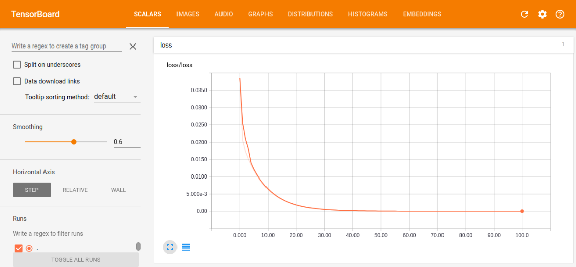
scalar中的loss训练图
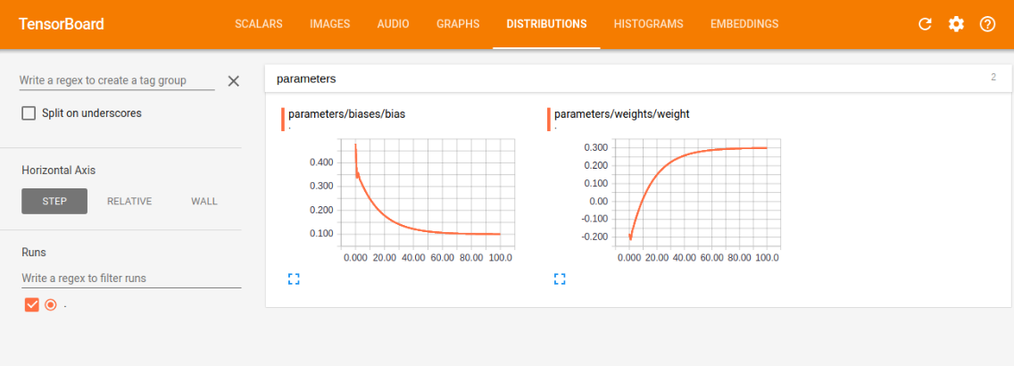
distribution中的weight和bias的训练图
histogram中的weight和bias的训练图

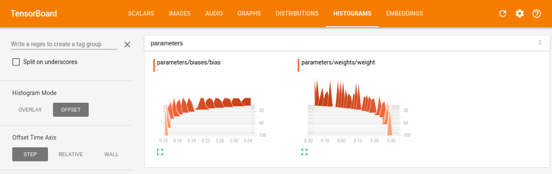
我们可以根据训练图，对学习情况进行评估，比如我们看损失训练图，可以看到现在是一条慢慢减小的曲线，最后的值趋近趋近于0（这里趋近于0是由于我选的模型太容易训练了，误差可以逼近0，同时又能很好的表征系统的模型，在现实情况，往往都有误差，趋近于0反而是过拟合），这符合本意，就是要最小化loss，如果loss的曲线最后没有平滑趋近一个数，则说明训练的力度还不够，还有加大次数，如果loss还很大，说明学习算法不太理想，需改变当前的算法，去实现更小的loss，另外两幅图与loss类似，最后都是要趋近一个数的，没有趋近和上下浮动都是有问题的。

3. 最后

欢迎大家扫一扫下面二维码加入微信交流群，如果二维码失效，可以添加博主个人微信，拉你进群

传送门----->Tensorflow系列教程