读西瓜书：7.1/7.2/7.3章

7.1 贝叶斯决策论

概率框架下是基于概率和误判损失来决策的

• 给定N个类别，令 $\lambda_{ij}$ 代表将第 $j$ 类样本误分为第 $i$ 类产生的损失，则基于后验概率将样本x分到第 $i$ 类的条件风险为

  • $R(c_i|x)=\sum_{j=1}^N\lambda_{ij}P(c_j|x) \tag{1}$

  • $\lambda_{ij}$ 通常为正，所以 (1) 式可以理解为当样本本属于第 $j$ 类的概率越大，那么将它分到第 $i$ 类所产生的损失越大

贝叶斯判定准则

• $h^*(x)=argmin_{c\in{y}}R(c|x) \tag{2}$
  • $h^*$ 称作贝叶斯最优分类器，其总体风险称为贝叶斯风险
  • 反应了学习性能的理论上限

判别式 vs. 生成式

• 后验概率 $P(c|x)$ 在现实中通常难以直接获得

  • 机器学习可以从这个角度看作是基于有限的训练样本尽可能准确估计出后验概率

• 两种基本策略

  • 	判别式模型	生成式模型
    思路	对 $P(c$| $x)$ 建模	对 $P(x,c)$ 建模
    代表	决策树，SVM	贝叶斯分类器

  • 注：prml 中还分了判别函数策略，其实属于判别式模型，因为 $P(c|x)$就是一个关于 $x$ 的函数

贝叶斯定理

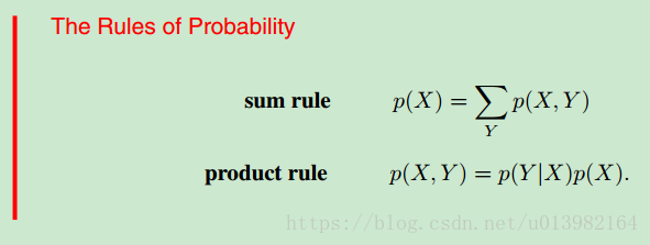
• (补充，来自PRML 第一章)首先我们介绍机器学习里概率论中最重要的两个公式如下

-

• Here $p(X, Y )$ is a joint probability and is verbalized as “the probability of X and Y ”. Similarly, the quantity $p(Y |X)$ is a conditional probability and is verbalized as “the probability of Y given X”, whereas the quantity $p(X)$ is a marginal probability and is simply “the probability of X”. These two simple rules form the basis for all of the probabilistic machinery that we use throughout this book

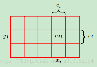
• 理解这两个公式最简单的就是数格子，如下图

• 

• sum rule

  • The probability that X will take the value xi and Y will take the value yj is written $p(X = x_i, Y = y_j)$ and is called the joint probability of $X = x_i$ and $Y = y_j$. It is given by the number of points falling in the cell $ i,j $ as a fraction of the total number of points, and hence
  • $p(X=x_i , Y=y_i)=\frac{n_{ij}}{N} \tag{3}$
  • Here we are implicitly considering the limit $N → ∞.$ Similarly, the probability that X takes the value xi irrespective of the value of $Y$ is written as $p(X = x_i)$ and is given by the fraction of the total number of points that fall in column i, so that
  • $p(X=x_i)=\frac{c_i}{N} \tag{4}$
  • 其中 $c_i = \sum_jn_{ij} $ , 根据 (3~4) 可以推出 sum rule:
  • $p(X=x_i)=\frac{c_i}{N}=\frac{\sum_jn_{ij}}{N}=\sum_j\frac{n_{ij}}{N}=\sum_jp(X=x_i , Y=y_i) \tag{5}$
  • Note that $p(X = x_i)$ is sometimes called the marginal probability, because it is obtained by marginalizing, or summing out, the other variables (in this case $Y$ ).

• product rule

  • If we consider only those instances for which $X = x_i$, then the fraction of such instances for which $Y = y_j$ is written $p(Y = y_j|X = x_i$) and is called the conditional probability of $Y = y_j$ given $X = x_i$. It is obtained by finding the fraction of those points in column $i$ that fall in cell $i,j$ and hence is given by
  • $p(Y=y_j|X=x_i)=\frac{n_{ij}}{c_i} \tag{6}$
  • 根据 (3, 4, 6)可以推出 product rule:
  • $p(X = x_i, Y = y_j) =\frac{n_{ij}}{N}=\frac{n_ij}{c_i}·\frac{c_i}{N} =p(Y=y_j|X=x_i)p(X=x_i) \tag{7}$

• 用以上两个公式其实就能推出贝叶斯公式

  • From the product rule, together with the symmetry property $p(X, Y ) = p(Y, X)$, we immediately obtain the following relationship between conditional probabilities
    - $p(X, Y ) = p(Y, X) \\p(X|Y)p(Y)=p(Y|X)p(X) \\ \frac{p(X|Y)p(Y)}{p(X)}=p(Y|X) \\p(Y|X)= \frac{p(X|Y)p(Y)}{\sum_Yp(X|Y)p(Y)} \tag{8}$
  • which is called Bayes’ theorem and which plays a central role in pattern recognition and machine learning
    • 其中 $p(Y)$ 是先验概率：样本空间中各类样本所占的比例，可通过各类样本出现的频率估计（大数定律）
    • $p(X)$ 是证据因子，与类别无关，可以当成起归一化的作用
    • $p(X|Y)$ 是样本相对于类标记的类条件概率，也叫似然
    • 由于 $p(X|Y)$ 涉及关于 $x$ 所有属性的联合概率，不能直接根据样本出现频率来估计，因为“未被观测到”与“出现概率为零”通常是不同的，所以主要困难在于估计似然 $p(X|Y)$

7.2 极大似然估计

如果是回归问题， Minimizing sum of square error is the same as maximum likelihood
solution under a Gaussian noise model

概率统计角度：

• 问题：已有一堆数据从某个概率分布中产生的，这个分布存在参数，我们目标是把参数估计出来

• 极大似然的思想：频率派认为观测到的样本肯定在原分布中出现的概率非常大（很好理解，在同一个分布中，只有概率特别大，才容易被采样出来嘛），所以做法是让估计出来的参数在观测数据上的联合概率尽可能大，而这个联合概率就叫似然。

• 做法：先假设某种概率分布形式，再基于训练样本对参数进行估计

  • 假定 $P(x|c)$ 具有确定的概率分布形式，且被参数 $\theta_c$ 唯一确定，则任务就是用训练集 $D$ 来估计参数 $\theta_c$

  • 记 $P(x|c)$ 为 $P(x|\theta_c)$， $\theta_c$ 对于训练集 $D$ 中第 $c$ 类样本组成的集合 $D_c$ 的似然为

    $P(D_c|\theta_c)=\prod_{x\in{D_C}} P(x|\theta_c) \tag{9}$
    注意这里假设每个样本都是独立产生的

  • 因为连乘在计算机中容易造成下溢 (数值分析) ，因此通常使用对数似然 $LL(\theta_c)=logP(D_c|\theta_c) = \sum_{x\in{D_c}}logP(x|\theta_c) \tag{10}$

  • 所以 $\theta_c$ 的MLE为 $\hat{\theta_c}=argmax_{\theta_c}LL(\theta_c) \tag{11}$

  • 估计结果的准确性严重依赖于所假设的概率分布形式是否符合潜在的真实分布

  • 可能会出现所要估计的概率为 0 的情况 ，影响后验概率的计算结果

• （补充，来自模式分类 第三章）数估计有两类方法

  • 将参数作为非随机量处理，如矩法估计、极大似然估计；

  • 将参数作为随机变量，如贝叶斯估计

    • 贝叶斯估计思想：引入损失函数 (1) 式，使所估计的 $\hat\theta_c$ 的使估计损失的期望最小

    • 步骤：

      1. 确定未知参数集 $\theta$ 的先验概密 $p(\theta_c)$
      2. 由样本集 $D_c$ 求 $P(D_c|\theta_c)$
      3. 由贝叶斯公式计算 $P(\theta_c | D_c)$
      4. 估计 $\hat\theta_c$：在观测 $D_c$ 条件下的 $\theta$ 的条件期望

    • 极大似然估计是贝叶斯估计的一个特例

7.3 朴素贝叶斯分类器

• 由于在有限训练样本上直接估计联合概率，在计算上会遭遇组合爆炸，数据上会遭遇样本稀疏的问题，朴素贝叶斯假设
  • 每个属性独立地对分类结果产生影响
  • 每个特征同等重要
  • 则贝叶斯公式可以重写为 $P(c|x)=\frac{P(c)P(x|c)}{P(x)}=\frac{P(c)}{P(x)}\prod^d_{i=1}P(x_i|c) \tag{12}$
  • 其中 $d$ 为特征数， $x_i$ 为 $x$ 在第 $i$ 个特征上的取值
• 因为 $P(x)$ 对所有类别相同，于是基于 (2) 式的贝叶斯判定准则有 $h_{nb}(x)=argmax_{c\in{y}}P(c)\prod^d_{i=1}P(x_i|c) \tag{13}$
  • 上式就是朴素贝叶斯分类器的表达式
• 朴素贝叶斯分类器的训练过程就是给定数据集D，来估计类先验概率 $P(c)$，及每个特征的条件概率 $P(x_i|c)$

总结

待续……

参考
周志华. 机器学习. 7.1/7.2/7.3.
Bishop. Pattern Recognition And Machine Learning. 1.2.
李宏东. 模式分类（译）. 3.