LDA是一种监督学习的数据降维方式:
将带有标签的数据降维,投影到低维空间同时满足三个条件:
- 尽可能多地保留数据样本的信息(即选择最大的特征是对应的特征向量所代表的的方向)。
- 寻找使样本尽可能好分的最佳投影方向。
- 投影后使得同类样本尽可能近,不同类样本尽可能远
1.LDA原理详解
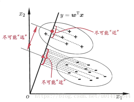
将样例投影到一条直线上,使得同类样本尽可能接近,异类样本尽可能远离。
给定数据集一共有C类样本,样本总数为M, 第i类有Mi个样本 第i类样本的均值 ui 所有样本的均值向量u 第i类样本的协方差矩阵
直线w
将数据投影到直线上 样本中心有
所有样本投影到直线上,样本的协方差
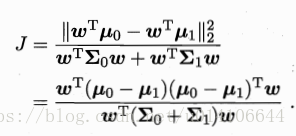
同类样本尽可能接近,即要小 异类样本尽可能远离,即
要大,有:
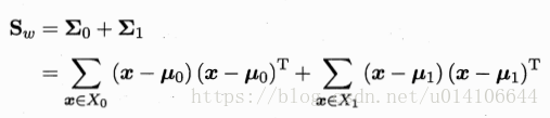
类内散度矩阵:
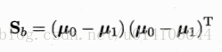
类间散度矩阵:

以上是LDA最大化的目标,为Sb,Sw是广义瑞利商。
分子分母都是关于w的二次函数,因此最终结果与w的长度无关,只与其方向有关。

拉格朗日乘数法:
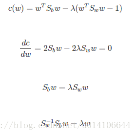
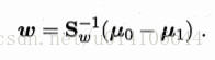
Sbw方向恒为 u0-u1 令:

最终结果求解如下;一般先对Sw进行奇异值分解,然后求解w
类似应用于多分类:
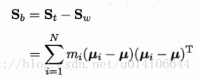
类内散度矩阵为每个类别的散度矩阵之和:


全局散度矩阵:

类间散度矩阵:
优化目标:
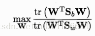
W的解是Sw的逆*Sb的N-1个最大特征值对应的特征向量构成的矩阵。
2.编程实现LDA
以下为例:
http://sebastianraschka.com/Articles/2014_python_lda.html
数据集文件格式如下所示:
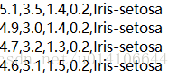
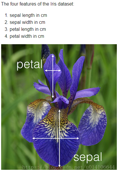
特征4个
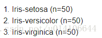
类别有3类
1. 加载数据集分析数据
loaddata() 结果返回特征向量矩阵X以及类别列向量y
def loaddata():
	feature_dict = {i:label for i,label in zip(
				range(4),
				  ('sepal length in cm',
				  'sepal width in cm',
				  'petal length in cm',
				  'petal width in cm', ))}
	df = pd.io.parsers.read_csv(
		filepath_or_buffer='https://archive.ics.uci.edu/ml/machine-learning-databases/iris/iris.data',
		header=None,
		sep=',',
		)
	df.columns = [l for i,l in sorted(feature_dict.items())] + ['class label']
	df.dropna(how="all", inplace=True) # to drop the empty line at file-end
	df.tail()

	from sklearn.preprocessing import LabelEncoder
	#取出前四列特征向量
	X = df[['sepal length in cm',
                  'sepal width in cm',
                  'petal length in cm',
                  'petal width in cm']].values
    #取出类别向量
	y = df['class label'].values
	enc = LabelEncoder()
	label_encoder = enc.fit(y)
	y = label_encoder.transform(y) + 1
	return X,y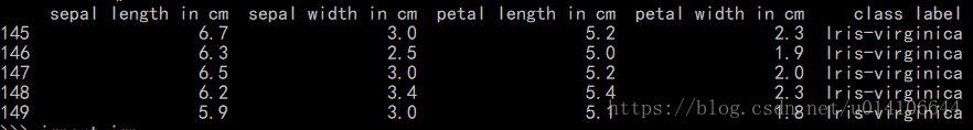
处理数据,观察数据在各个特征向量中类别分布信息:
错误,TAB键改成4个空格:

代码如下:
def showdata(X, y):
    from matplotlib import pyplot as plt
    import numpy as np
    import math
    label_dict = {1: 'Setosa', 2: 'Versicolor', 3:'Virginica'}
    fig, axes = plt.subplots(nrows=2, ncols=2, figsize=(12,6))
    for ax,cnt in zip(axes.ravel(), range(4)):
	    # set bin sizes
	    min_b = math.floor(np.min(X[:,cnt]))
	    max_b = math.ceil(np.max(X[:,cnt]))
	    bins = np.linspace(min_b, max_b, 25)
	    # plottling the histograms
	    for lab,col in zip(range(1,4), ('blue', 'red', 'green')):
		    ax.hist(X[y==lab, cnt],
				   color=col,
				   label='class %s' %label_dict[lab],
				   bins=bins,
				   alpha=0.5,)
	    ylims = ax.get_ylim()
	    # plot annotation
	    leg = ax.legend(loc='upper right', fancybox=True, fontsize=8)
	    leg.get_frame().set_alpha(0.5)
	    ax.set_ylim([0, max(ylims)+2])
	    ax.set_xlabel(feature_dict[cnt])
	    ax.set_title('Iris histogram #%s' %str(cnt+1))
	    # hide axis ticks
	    ax.tick_params(axis="both", which="both", bottom="off", top="off",
			labelbottom="on", left="off", right="off", labelleft="on")
	    # remove axis spines
	    ax.spines["top"].set_visible(False)
	    ax.spines["right"].set_visible(False)
	    ax.spines["bottom"].set_visible(False)
	    ax.spines["left"].set_visible(False)
    axes[0][0].set_ylabel('count')
    axes[1][0].set_ylabel('count')
    fig.tight_layout()
    plt.show()
显示结果如下:
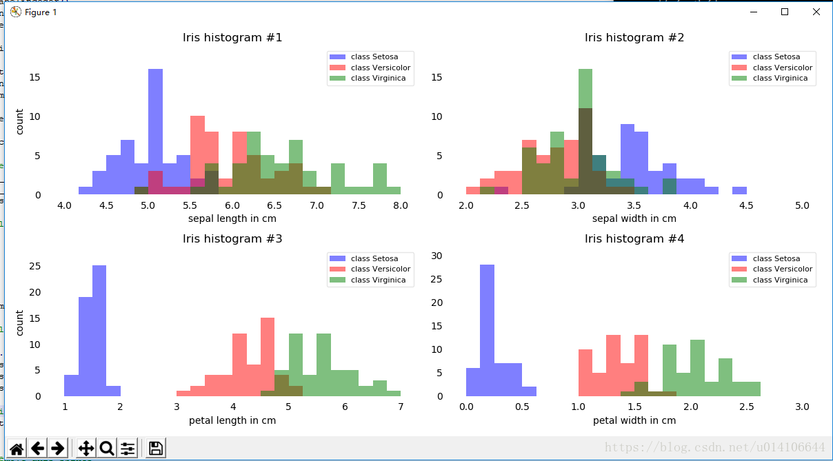
由以上可知数据在属性petal length width方向上由很好的类别区分度。
2.LDA分析计算
Step 1: Computing the d-dimensional mean vectors 计算各种类别均值 ui
def meanvector(X, y):
    np.set_printoptions(precision=4)
    mean_vectors = []
    for cl in range(1,4):
        mean_vectors.append(np.mean(X[y==cl], axis=0))
        print('Mean Vector class %s: %s\n' %(cl, mean_vectors[cl-1]))
    return mean_vectors
Step 2: Computing the Scatter Matrices 计算散度矩阵
类内散度矩阵计算
def within_class_scatter(X, y, mean_vectors):
    S_W = np.zeros((4,4))
    for cl,mv in zip(range(1,4), mean_vectors):
        class_sc_mat = np.zeros((4,4))                  # scatter matrix for every class
        for row in X[y == cl]:
            row, mv = row.reshape(4,1), mv.reshape(4,1) # make column vectors
            class_sc_mat += (row-mv).dot((row-mv).T)
        S_W += class_sc_mat                             # sum class scatter matrices
    print('within-class Scatter Matrix:\n', S_W)
    return S_W
类间散度矩阵计算
def between_class_scatter(X, y, mean_vectors):
    overall_mean = np.mean(X, axis=0)
    S_B = np.zeros((4,4))
    for i,mean_vec in enumerate(mean_vectors):
        n = X[y==i+1,:].shape[0]
        mean_vec = mean_vec.reshape(4,1) # make column vector
        overall_mean = overall_mean.reshape(4,1) # make column vector
        S_B += n * (mean_vec - overall_mean).dot((mean_vec - overall_mean).T)
    print('between-class Scatter Matrix:\n', S_B)
    return S_B
Step 3: Solving the generalized eigenvalue problem for the matrix 求解特征值分解
def eigenvalue(S_W, S_B):
    eig_vals, eig_vecs = np.linalg.eig(np.linalg.inv(S_W).dot(S_B))
    for i in range(len(eig_vals)):
        eigvec_sc = eig_vecs[:,i].reshape(4,1)
        print('\nEigenvector {}: \n{}'.format(i+1, eigvec_sc.real))
        print('Eigenvalue {:}: {:.2e}'.format(i+1, eig_vals[i].real))
    return eig_vals, eig_vecs
进行特征值和特征向量的求解。
Step 4: Selecting linear discriminants for the new feature subspace
对特征向量以特征值进行降序排序
def sortvec(eig_vals, eig_vecs):
    # Make a list of (eigenvalue, eigenvector) tuples
    eig_pairs = [(np.abs(eig_vals[i]), eig_vecs[:,i]) for i in range(len(eig_vals))]
    # Sort the (eigenvalue, eigenvector) tuples from high to low
    eig_pairs = sorted(eig_pairs, key=lambda k: k[0], reverse=True)
    # Visually confirm that the list is correctly sorted by decreasing eigenvalues
    print('Eigenvalues in decreasing order:\n')
    for i in eig_pairs:
        print(i[0])
    return eig_pairs
返回最大的k个特征值对应的特征向量组成的矩阵,即为W
def getW(eig_pairs):
    W = np.hstack((eig_pairs[0][1].reshape(4,1), eig_pairs[1][1].reshape(4,1)))
    print('Matrix W:\n', W.real)
    return W
Step 5: Transforming the samples onto the new subspace
将样本转为到W的向量空间内,实现了降维操作。并绘出样本分布图
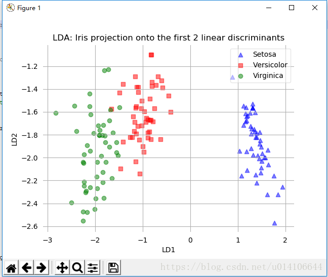
在LD1维度上,样本实现了很好的分类。
LDA降维的过程就是对于矩阵的特征值分解,取其最大的k个特征值对应的向量来组成W,从而实现数据的降维处理。之后会与PCA降维分解进行比较:PCA是为了去除原始数据集中冗余的维度,让投影子空间的各个维度的方差尽可能大,也就是熵尽可能大,无监督学习。LDA是通过数据降维找到那些具有discriminative的维度,使得原始数据在这些维度上的投影,不同类别尽可能区分开来,有监督学习。