目录
引言
极限学习机不是一个新的东西,只是在算法(方法)上有新的内容。在神经网络结构上,就是一个前向传播的神经网络,和之前几篇博文讲的意义。

为什么我们需要ELM?
The learning speed of feedforward neural networks is in general far slower than required and it has been a major bottleneck in their applications for past decades. Two key reasons behind may be:
1) the slow gradient-based learning algorithms are extensively used to train neural networks.
2) all the parameters of the networks are tuned iteratively by using such learning algorithms.
最大的创新点:
1)输入层和隐含层的连接权值、隐含层的阈值可以随机设定,且设定完后不用再调整。这和BP神经网络不一样,BP需要不断反向去调整权值和阈值。因此这里就能减少一半的运算量了。
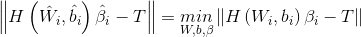
2)隐含层和输出层之间的连接权值β不需要迭代调整,而是通过解方程组方式一次性确定。
研究表明,通过这样的规则,模型的泛化性能很好,速度提高了不少。
一言概之,ELM最大的特点就是对于传统的神经网络,尤其是单隐层前馈神经网络(SLFNs),在保证学习精度的前提下比传统的学习算法速度更快。
Compared BP Algorithm and SVM,ELM has several salient features:
•Ease of use. No parameters need to be manually tuned except predefined network architecture.只有隐含层神经元个数需要我们调整。
•Faster learning speed. Most training can be completed in milliseconds, seconds, and minutes.
•Higher generalization performance. It could obtain better generalization performance than BP in most cases, and reach generalization performance similar to or better than SVM.(泛化能力提升)
•Suitable for almost all nonlinear activation functions.Almost all piecewise continuous (including discontinuous, differential, non-differential functions) can be used as activation functions.
•Suitable for fully complex activation functions. Fully complex functions can also be used as activation functions in ELM.
极限学习机原理
ELM是一种新型的快速学习算法,对于单隐层神经网络,ELM可以随机初始化输入权重和偏置并得到相应的输出权重。
对于一个单隐层神经网络(见上面的图),假设有


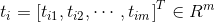

其中,


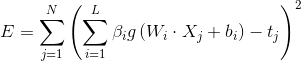
单隐层神经网络学习的目标是使得输出的误差最小,可以表示为
即存在


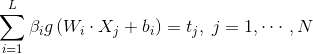
可以矩阵表示为

其中,


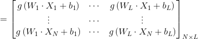
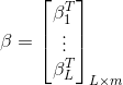
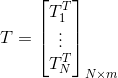
为了能够训练单隐层神经网络,我们希望得到


其中,
传统的一些基于梯度下降法的算法,可以用来求解这样的问题,但是基本的基于梯度的学习算法需要在迭代的过程中调整所有参数。而在ELM算法中, 一旦输入权重


其中,


上面涉及到矩阵论的一些知识,其实也不需要理解,只要百度一下相关的概念,比如广义逆怎么求,或直接matlab里面去算就好了。对于偏工程应用的人而言,此处不需要多费时间了解数学原理。
ELM的作者,黄广斌老师提供的代码:http://www.ntu.edu.sg/home/egbhuang/elm_codes.html
参考博文:https://blog.csdn.net/google19890102/article/details/18222103?utm_source=copy
MATLAB中重点函数解读
下面我们打算用MATLAB来实现以下ELM。使用到的不是作者的代码,而是网络上的高手前辈们自己写的代码。
-
nargin:n arg in:自动计算出方法输入了几个参数
-
error:给出错误信息
-
pinv:求伪逆矩阵
-
sin / hardlim:涉及到激活函数
-
elmtrain 自己写的函数,用于ELM训练,记住:每一列代表一个样本
function [IW,B,LW,TF,TYPE] = elmtrain(P,T,N,TF,TYPE)
% ELMTRAIN Create and Train a Extreme Learning Machine
% Syntax
% [IW,B,LW,TF,TYPE] = elmtrain(P,T,N,TF,TYPE)
% Description
% Input
% P   - Input Matrix of Training Set  (R*Q)
% T   - Output Matrix of Training Set (S*Q)
% N   - Number of Hidden Neurons (default = Q)
% TF  - Transfer Function:
%       'sig' for Sigmoidal function (default)
%       'sin' for Sine function
%       'hardlim' for Hardlim function
% TYPE - Regression (0,default) or Classification (1)
% Output
% IW  - Input Weight Matrix (N*R)
% B   - Bias Matrix  (N*1)
% LW  - Layer Weight Matrix (N*S)
% Example
% Regression:
% [IW,B,LW,TF,TYPE] = elmtrain(P,T,20,'sig',0)
% Y = elmtrain(P,IW,B,LW,TF,TYPE)
% Classification
% [IW,B,LW,TF,TYPE] = elmtrain(P,T,20,'sig',1)
% Y = elmtrain(P,IW,B,LW,TF,TYPE)
% See also ELMPREDICT
% Yu Lei,11-7-2010
% Copyright www.matlabsky.com
% $Revision:1.0 $
if nargin < 2
    error('ELM:Arguments','Not enough input arguments.');
end
if nargin < 3
    N = size(P,2);
end
if nargin < 4
    TF = 'sig';
end
if nargin < 5
    TYPE = 0;
end
if size(P,2) ~= size(T,2)
    error('ELM:Arguments','The columns of P and T must be same.');
end
[R,Q] = size(P);
if TYPE  == 1
    T  = ind2vec(T);
end
[S,Q] = size(T);
% Randomly Generate the Input Weight Matrix
IW = rand(N,R) * 2 - 1;
% Randomly Generate the Bias Matrix
B = rand(N,1);
BiasMatrix = repmat(B,1,Q);
% Calculate the Layer Output Matrix H
tempH = IW * P + BiasMatrix;
switch TF
    case 'sig'
        H = 1 ./ (1 + exp(-tempH));
    case 'sin'
        H = sin(tempH);
    case 'hardlim'
        H = hardlim(tempH);
end
% Calculate the Output Weight Matrix
LW = pinv(H') * T';
-
elmpredict 自己写的函数
function [IW,B,LW,TF,TYPE] = elmtrain(P,T,N,TF,TYPE)
% ELMTRAIN Create and Train a Extreme Learning Machine
% Syntax
% [IW,B,LW,TF,TYPE] = elmtrain(P,T,N,TF,TYPE)
% Description
% Input
% P   - Input Matrix of Training Set  (R*Q)
% T   - Output Matrix of Training Set (S*Q)
% N   - Number of Hidden Neurons (default = Q)
% TF  - Transfer Function:
%       'sig' for Sigmoidal function (default)
%       'sin' for Sine function
%       'hardlim' for Hardlim function
% TYPE - Regression (0,default) or Classification (1)
% Output
% IW  - Input Weight Matrix (N*R)
% B   - Bias Matrix  (N*1)
% LW  - Layer Weight Matrix (N*S)
% Example
% Regression:
% [IW,B,LW,TF,TYPE] = elmtrain(P,T,20,'sig',0)
% Y = elmtrain(P,IW,B,LW,TF,TYPE)
% Classification
% [IW,B,LW,TF,TYPE] = elmtrain(P,T,20,'sig',1)
% Y = elmtrain(P,IW,B,LW,TF,TYPE)
% See also ELMPREDICT
% Yu Lei,11-7-2010
% Copyright www.matlabsky.com
% $Revision:1.0 $
if nargin < 2
    error('ELM:Arguments','Not enough input arguments.');
end
if nargin < 3
    N = size(P,2);
end
if nargin < 4
    TF = 'sig';
end
if nargin < 5
    TYPE = 0;
end
if size(P,2) ~= size(T,2)
    error('ELM:Arguments','The columns of P and T must be same.');
end
[R,Q] = size(P);
if TYPE  == 1
    T  = ind2vec(T);
end
[S,Q] = size(T);
% Randomly Generate the Input Weight Matrix
IW = rand(N,R) * 2 - 1;
% Randomly Generate the Bias Matrix
B = rand(N,1);
BiasMatrix = repmat(B,1,Q);
% Calculate the Layer Output Matrix H
tempH = IW * P + BiasMatrix;
switch TF
    case 'sig'
        H = 1 ./ (1 + exp(-tempH));
    case 'sin'
        H = sin(tempH);
    case 'hardlim'
        H = hardlim(tempH);
end
% Calculate the Output Weight Matrix
LW = pinv(H') * T';
极限学习机的MATLAB实践
【实例1】汽油辛烷值预测
%% I. 清空环境变量
clear all
clc

%% II. 训练集/测试集产生
%%
% 1. 导入数据
load spectra_data.mat

%%
% 2. 随机产生训练集和测试集
temp = randperm(size(NIR,1));

% 训练集――50个样本
P_train = NIR(temp(1:50),:)';
T_train = octane(temp(1:50),:)';

% 测试集――10个样本
P_test = NIR(temp(51:end),:)';
T_test = octane(temp(51:end),:)';
N = size(P_test,2);

%% III. 数据归一化
%%
% 1. 训练集
[Pn_train,inputps] = mapminmax(P_train);
Pn_test = mapminmax('apply',P_test,inputps);
%%
% 2. 测试集
[Tn_train,outputps] = mapminmax(T_train);
Tn_test = mapminmax('apply',T_test,outputps);

%% IV. ELM创建/训练
[IW,B,LW,TF,TYPE] = elmtrain(Pn_train,Tn_train,30,'sig',0);

%% V. ELM仿真测试
tn_sim = elmpredict(Pn_test,IW,B,LW,TF,TYPE);
%%
% 1. 反归一化
T_sim = mapminmax('reverse',tn_sim,outputps);

%% VI. 结果对比
result = [T_test' T_sim'];
%%
% 1. 均方误差
E = mse(T_sim - T_test);

%%
% 2. 决定系数
N = length(T_test);
R2=(N*sum(T_sim.*T_test)-sum(T_sim)*sum(T_test))^2/((N*sum((T_sim).^2)-(sum(T_sim))^2)*(N*sum((T_test).^2)-(sum(T_test))^2));

%% VII. 绘图
figure(1)
plot(1:N,T_test,'r-*',1:N,T_sim,'b:o')
grid on
legend('真实值','预测值')
xlabel('样本编号')
ylabel('辛烷值')
string = {'测试集辛烷值含量预测结果对比(ELM)';['(mse = ' num2str(E) ' R^2 = ' num2str(R2) ')']};
title(string)
【实例2】鸢尾花侯种类识别
%% I. 清空环境变量
clear all
clc

%% II. 训练集/测试集产生
%%
% 1. 导入数据
load iris_data.mat

%%
% 2. 随机产生训练集和测试集
P_train = [];
T_train = [];
P_test = [];
T_test = [];
for i = 1:3
    temp_input = features((i-1)*50+1:i*50,:);
    temp_output = classes((i-1)*50+1:i*50,:);
    n = randperm(50);
    % 训练集――120个样本
    P_train = [P_train temp_input(n(1:40),:)'];
    T_train = [T_train temp_output(n(1:40),:)'];
    % 测试集――30个样本
    P_test = [P_test temp_input(n(41:50),:)'];
    T_test = [T_test temp_output(n(41:50),:)'];
end

%% III. ELM创建/训练
[IW,B,LW,TF,TYPE] = elmtrain(P_train,T_train,20,'sig',1);

%% IV. ELM仿真测试
T_sim_1 = elmpredict(P_train,IW,B,LW,TF,TYPE);
T_sim_2 = elmpredict(P_test,IW,B,LW,TF,TYPE);

%% V. 结果对比
result_1 = [T_train' T_sim_1'];
result_2 = [T_test' T_sim_2'];
%%
% 1. 训练集正确率
k1 = length(find(T_train == T_sim_1));
n1 = length(T_train);
Accuracy_1 = k1 / n1 * 100;
disp(['训练集正确率Accuracy = ' num2str(Accuracy_1) '%(' num2str(k1) '/' num2str(n1) ')'])

%%
% 2. 测试集正确率
k2 = length(find(T_test == T_sim_2));
n2 = length(T_test);
Accuracy_2 = k2 / n2 * 100;
disp(['测试集正确率Accuracy = ' num2str(Accuracy_2) '%(' num2str(k2) '/' num2str(n2) ')'])

%% VI. 绘图
figure(2)
plot(1:30,T_test,'bo',1:30,T_sim_2,'r-*')
grid on
xlabel('测试集样本编号')
ylabel('测试集样本类别')
string = {'测试集预测结果对比(ELM)';['(正确率Accuracy = ' num2str(Accuracy_2) '%)' ]};
title(string)
legend('真实值','ELM预测值')