SRCNN_小结

SRCNN Super-Resolution Convolutional Neural Network (超分辨率重建卷积神经网络)，网络模型如图所示：

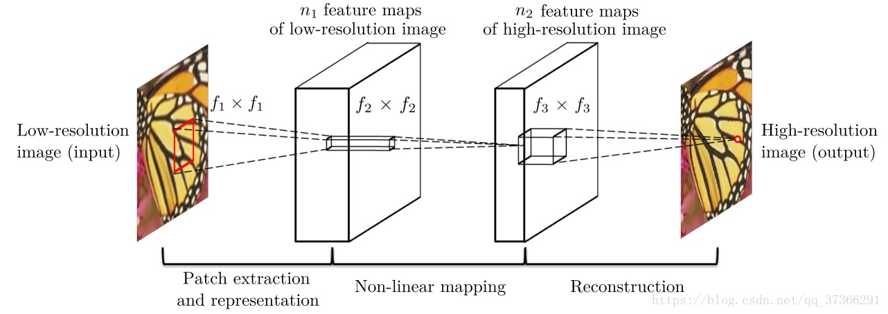
该方法对于一个低分辨率图像，先使用双三次（bicubic）插值将其放大到目标大小，再通过三层卷积网络做非线性映射，得到的结果作为高分辨率图像输出。作者将三层卷积的结构解释成与传统SR方法对应的三个步骤：图像块的提取和特征表示，特征非线性映射和最终的重建。

三个卷积层使用的卷积核的大小分为为9x9, 1x1和5x5，前两个的输出特征个数分别为64和32. 该文章分别用Timofte数据集（包含91幅图像）和ImageNet大数据集进行训练。相比于双三次插值和传统的稀疏编码方法，SRCNN得到的高分辨率图像更加清晰。

对SR的质量进行定量评价常用的两个指标是PSNR(Peak Signal-to-Noise Ratio)和SSIM（Structure Similarity Index）。这两个值越高代表重建结果的像素值和原标准越接近。后面我们会知道：卷积神经网络的代价函数就是PSNR的取值。

实验环境：caffe , Ubuntu 14.04.5 LTS，实验代码。我们要先在官网上下载caffe的源代码。通过cmake进行编译。生成可执行文件。这里涉及很多c语言的知识，因为caffe是用c语言写的，我在这里还留下很多不知道的坑，嗯，希望我以后可以慢慢全部搞懂。
训练看了很多资料感觉caffe是一个非常友好的框架。打个比方：如果说机器学习是炼丹，那么只需要知道大的过程就可以用caffe了。我们在caffe的根目录下输入：该命令就可以训练我们的模型了。

./build/tools/caffe train --solver=examples/SRCNN/SRCNN_solver.prototxt

SRCNN文件夹的内容是我们从github上下载的实验源代码。（装好git,一个命令就可以了。）我是从window上的cmd命令去理解这个命令的。./build/tools/caffe = 相对路径 + 可执行文件名（其实我们花那么大功夫去编译caffe也就是得到这个caffe）.
train solver=examples/SRCNN/SRCNN_solver.prototxt ，相当于参数赋值。

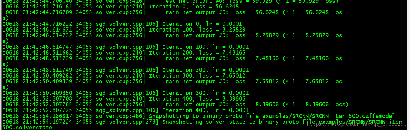
上图是：训练过程的结果显示。解释一些参数：
Iteration 0 迭代次数为0次
lr = 0.0001 学习率。（具体作用：反向传播，梯度下降时的迭代因子）
loss = 8.25829 代价函数的取值。
注意到当迭代次数达到500时，会显示

I0618 21:42:54.186817 34055 solver.cpp:466] Snapshotting to binary proto file examples/SRCNN/SRCNN_iter_500.caffemodel
I0618 21:42:54.197224 34055 sgd_solver.cpp:273] Snapshotting solver state to binary proto file examples/SRCNN/SRCNN_iter_500.solverstate

这些内容是提示我们，训练500次的模型结果保存的路径。同样的这个参数我们也可以设置，下面会说。你看其实到这里caffe的训练过程就完成。当然还有很多细节之处我们不知道。首先我们传给caffe的参数 SRCNN_solver.prototxt 文件里写了什么？
SRCNN_solver.prototxt

# The train/test net protocol buffer definition
net: "examples/SRCNN/SRCNN_net.prototxt"    # 网络结构的描述文件
test_iter: 556 
# Carry out testing every 500 training iterations.
test_interval: 500
# The base learning rate, momentum and the weight decay of the network.
base_lr: 0.0001
momentum: 0.9
weight_decay: 0
# The learning rate policy
lr_policy: "fixed"
# Display every 100 iterations
display: 100
# The maximum number of iterations
max_iter: 15000000
# snapshot intermediate results
snapshot: 500
snapshot_prefix: "examples/SRCNN/SRCNN"
# solver mode: CPU or GPU
solver_mode: GPU

我们可以发现：有些参数在我们训练的过程已经有所体现。base_lr，snapshot…..

这里第一行的参数非常重要。net: “examples/SRCNN/SRCNN_net.prototxt”，这个是我们的核心文件，里边描述了具体的网络层次。

name: "SRCNN"
layer {
  name: "data"
  type: "HDF5Data"
  top: "data"
  top: "label"
  hdf5_data_param {
    source: "examples/SRCNN/train.txt"
    batch_size: 128
  }
  include: { phase: TRAIN }
}
layer {
  name: "data"
  type: "HDF5Data"
  top: "data"
  top: "label"
  hdf5_data_param {
    source: "examples/SRCNN/test.txt"
    batch_size: 2
  }
  include: { phase: TEST }
}

layer {
  name: "conv1"
  type: "Convolution"
  bottom: "data"
  top: "conv1"
  param {
    lr_mult: 1
  }
  param {
    lr_mult: 0.1
  }
  convolution_param {
    num_output: 64
    kernel_size: 9
    stride: 1
    pad: 0
    weight_filler {
      type: "gaussian"
      std: 0.001
    }
    bias_filler {
      type: "constant"
      value: 0
    }
  }
}

layer {
  name: "relu1"
  type: "ReLU"
  bottom: "conv1"
  top: "conv1"
}

layer {
  name: "conv2"
  type: "Convolution"
  bottom: "conv1"
  top: "conv2"
  param {
    lr_mult: 1
  }
  param {
    lr_mult: 0.1
  }
  convolution_param {
    num_output: 32
    kernel_size: 1
    stride: 1
    pad: 0
    weight_filler {
      type: "gaussian"
      std: 0.001
    }
    bias_filler {
      type: "constant"
      value: 0
    }
  }
}

layer {
  name: "relu2"
  type: "ReLU"
  bottom: "conv2"
  top: "conv2"
}

layer {
  name: "conv3"
  type: "Convolution"
  bottom: "conv2"
  top: "conv3"
  param {
    lr_mult: 0.1
  }
  param {
    lr_mult: 0.1
  }
  convolution_param {
    num_output: 1
    kernel_size: 5
    stride: 1
    pad: 0
    weight_filler {
      type: "gaussian"
      std: 0.001
    }
    bias_filler {
      type: "constant"
      value: 0
    }
  }
}

layer {
  name: "loss"
  type: "EuclideanLoss"
  bottom: "conv3"
  bottom: "label"
  top: "loss"
}

这里我们可以看到刚开始说的三层卷积神经网络：conv1，conv2，conv3。

demo_SR.m

close all;
clear all;

%% read ground truth image
im  = imread('Set5/butterfly_GT.bmp');
%im  = imread('Set14\zebra.bmp');

%% set parameters
up_scale = 4;
model = 'model/9-5-5(ImageNet)/x4.mat';
% up_scale = 3;
% model = 'model\9-3-5(ImageNet)\x3.mat';
% up_scale = 3;
% model = 'model\9-1-5(91 images)\x3.mat';
% up_scale = 2;
% model = 'model\9-5-5(ImageNet)\x2.mat'; 
% up_scale = 4;
% model = 'model\9-5-5(ImageNet)\x4.mat';

%% work on illuminance only
if size(im,3)>1
    im = rgb2ycbcr(im);
    im = im(:, :, 1);
end
im_gnd = modcrop(im, up_scale);
im_gnd = single(im_gnd)/255;

%% bicubic interpolation
im_l = imresize(im_gnd, 1/up_scale, 'bicubic');
im_b = imresize(im_l, up_scale, 'bicubic');

%% SRCNN
im_h = SRCNN(model, im_b);

%% remove border
im_h = shave(uint8(im_h * 255), [up_scale, up_scale]);
im_gnd = shave(uint8(im_gnd * 255), [up_scale, up_scale]);
im_b = shave(uint8(im_b * 255), [up_scale, up_scale]);

%% compute PSNR
psnr_bic = compute_psnr(im_gnd,im_b);
psnr_srcnn = compute_psnr(im_gnd,im_h);

%% show results
fprintf('PSNR for Bicubic Interpolation: %f dB\n', psnr_bic);
fprintf('PSNR for SRCNN Reconstruction: %f dB\n', psnr_srcnn);

figure, imshow(im_b); title('Bicubic Interpolation');
figure, imshow(im_h); title('SRCNN Reconstruction');

%imwrite(im_b, ['Bicubic Interpolation' '.bmp']);
%imwrite(im_h, ['SRCNN Reconstruction' '.bmp']);


im  = imread('Set5/butterfly_GT.bmp');
figure, imshow(im); title('origin image');
im_h = cat(3,im_h,im_gnd,im_b);
figure, imshow(im_h); title('SRCNN');

demo_SR.m是用我们训练好的model进行超分辨率重建。嗯，代码里大多数都是matlab的基础命令，耐心读就可以了。
im = rgb2ycbcr(im);的作用是：…..这个应该是超分辨率重建套路吧。
im_h = SRCNN(model, im_b)， SRCNN（）也是我们需要写的函数。里边进行的是通过model的三次卷积运算。
psnr_bic = compute_psnr(im_gnd,im_b) 是计算图像的PSNR。

数据转换
有些时候，我们的输入不是标准的图像，而是其它一些格式，比如：频谱图、特征向量等等，这种情况下LMDB、Leveldb以及ImageData layer等就不好使了，这时候我们就需要一个新的输入接口——HDF5Data.

其实我们可以这样理解，就是caffe训练的数据类型不是.bmp, .jpg(图片格式) 这里我们需要将图片转换成 “HDF5Data” 类型。 这里用到了两个函数
generate_test.m ， store2hdf5.m。
generate_test.m

clear;close all;
% settings
folder = 'Train';              
savepath = 'train.h5';         
size_input = 33;
size_label = 21;
scale = 3;
stride = 14;

%% initialization
data = zeros(size_input, size_input, 1, 1);
label = zeros(size_label, size_label, 1, 1);
padding = abs(size_input - size_label)/2;
count = 0;

%% generate data
filepaths = dir(fullfile(folder,'*.bmp'));

for i = 1 : length(filepaths)

    image = imread(fullfile(folder,filepaths(i).name));
    image = rgb2ycbcr(image);
    image = im2double(image(:, :, 1));

    im_label = modcrop(image, scale);
    [hei,wid] = size(im_label);
    im_input = imresize(imresize(im_label,1/scale,'bicubic'),[hei,wid],'bicubic');

    for x = 1 : stride : hei-size_input+1
        for y = 1 :stride : wid-size_input+1

            subim_input = im_input(x : x+size_input-1, y : y+size_input-1);
            subim_label = im_label(x+padding : x+padding+size_label-1, y+padding : y+padding+size_label-1);

            count=count+1;
            data(:, :, 1, count) = subim_input;
            label(:, :, 1, count) = subim_label;
        end
    end
end

order = randperm(count);
data = data(:, :, 1, order);
label = label(:, :, 1, order); 

%% writing to HDF5
chunksz = 128;
created_flag = false;
totalct = 0;

for batchno = 1:floor(count/chunksz)
    last_read=(batchno-1)*chunksz;
    batchdata = data(:,:,1,last_read+1:last_read+chunksz); 
    batchlabs = label(:,:,1,last_read+1:last_read+chunksz);

    startloc = struct('dat',[1,1,1,totalct+1], 'lab', [1,1,1,totalct+1]);
    curr_dat_sz = store2hdf5(savepath, batchdata, batchlabs, ~created_flag, startloc, chunksz); 
    created_flag = true;
    totalct = curr_dat_sz(end);
end
h5disp(savepath);

store2hdf5.m

function [curr_dat_sz, curr_lab_sz] = store2hdf5(filename, data, labels, create, startloc, chunksz)  
  % *data* is W*H*C*N matrix of images should be normalized (e.g. to lie between 0 and 1) beforehand
  % *label* is D*N matrix of labels (D labels per sample) 
  % *create* [0/1] specifies whether to create file newly or to append to previously created file, useful to store information in batches when a dataset is too big to be held in memory  (default: 1)
  % *startloc* (point at which to start writing data). By default, 
  % if create=1 (create mode), startloc.data=[1 1 1 1], and startloc.lab=[1 1]; 
  % if create=0 (append mode), startloc.data=[1 1 1 K+1], and startloc.lab = [1 K+1]; where K is the current number of samples stored in the HDF
  % chunksz (used only in create mode), specifies number of samples to be stored per chunk (see HDF5 documentation on chunking) for creating HDF5 files with unbounded maximum size - TLDR; higher chunk sizes allow faster read-write operations 

  % verify that format is right
  dat_dims=size(data);
  lab_dims=size(labels);
  num_samples=dat_dims(end);

  assert(lab_dims(end)==num_samples, 'Number of samples should be matched between data and labels');

  if ~exist('create','var')
    create=true;
  end


  if create
    %fprintf('Creating dataset with %d samples\n', num_samples);
    if ~exist('chunksz', 'var')
      chunksz=1000;
    end
    if exist(filename, 'file')
      fprintf('Warning: replacing existing file %s \n', filename);
      delete(filename);
    end      
    h5create(filename, '/data', [dat_dims(1:end-1) Inf], 'Datatype', 'single', 'ChunkSize', [dat_dims(1:end-1) chunksz]); % width, height, channels, number 
    h5create(filename, '/label', [lab_dims(1:end-1) Inf], 'Datatype', 'single', 'ChunkSize', [lab_dims(1:end-1) chunksz]); % width, height, channels, number 
    if ~exist('startloc','var') 
      startloc.dat=[ones(1,length(dat_dims)-1), 1];
      startloc.lab=[ones(1,length(lab_dims)-1), 1];
    end 
  else  % append mode
    if ~exist('startloc','var')
      info=h5info(filename);
      prev_dat_sz=info.Datasets(1).Dataspace.Size;
      prev_lab_sz=info.Datasets(2).Dataspace.Size;
      assert(prev_dat_sz(1:end-1)==dat_dims(1:end-1), 'Data dimensions must match existing dimensions in dataset');
      assert(prev_lab_sz(1:end-1)==lab_dims(1:end-1), 'Label dimensions must match existing dimensions in dataset');
      startloc.dat=[ones(1,length(dat_dims)-1), prev_dat_sz(end)+1];
      startloc.lab=[ones(1,length(lab_dims)-1), prev_lab_sz(end)+1];
    end
  end

  if ~isempty(data)
    h5write(filename, '/data', single(data), startloc.dat, size(data));
    h5write(filename, '/label', single(labels), startloc.lab, size(labels));  
  end

  if nargout
    info=h5info(filename);
    curr_dat_sz=info.Datasets(1).Dataspace.Size;
    curr_lab_sz=info.Datasets(2).Dataspace.Size;
  end
end

未完待续