结构分析
caffe分为
1. Solver
2. Net
3. Layer
4. Blob
四层结构.
Solver : 负责模型的求解
Net : 负责定义网络的结构
Layer: 负责每一层网络功能的具体实现
Blob : 则定义数据,负责数据在每一层之间的流动。
Blob
1. 简介
Blob是:
- 对处理数据的一层封装,用于在Caffe中通信传递。
- 也为CPU和GPU间提供同步能力
- 数学上,是一个N维的C风格的存储数组
- 总的来说,Caffe使用Blob来交流数据,其是Caffe中标准的数组与统一的内存接口,它是多功能的,在不同的应用场景具有不同的含义,如可以是:batches of images(图像), model parameters(模型参数), and derivatives for optimization(最优化的导数)等。
2. 源代码
/**
 * @brief A wrapper around SyncedMemory holders serving as the basic
 *        computational unit through which Layer%s, Net%s, and Solver%s
 *        interact.
 *
 * TODO(dox): more thorough description.
 */
template <typename Dtype>
class Blob {
 public:
  Blob()
       : data_(), diff_(), count_(0), capacity_(0) {}

  /// @brief Deprecated; use <code>Blob(const vector<int>& shape)</code>.
  explicit Blob(const int num, const int channels, const int height,
      const int width);
  explicit Blob(const vector<int>& shape);

  .....

 protected:
  shared_ptr<SyncedMemory> data_;
  shared_ptr<SyncedMemory> diff_;
  shared_ptr<SyncedMemory> shape_data_;
  vector<int> shape_;
  int count_;
  int capacity_;

  DISABLE_COPY_AND_ASSIGN(Blob);
};  // class Blob
- 1
- 2
- 3
- 4
- 5
- 6
- 7
- 8
- 9
- 10
- 11
- 12
- 13
- 14
- 15
- 16
- 17
- 18
- 19
- 20
- 21
- 22
- 23
- 24
- 25
- 26
- 27
- 28
- 29
- 30
注:此处只保留了构造函数与成员变量。
说明:
- Blob在实现上是对SyncedMemory进行了一层封装。
- shape_为blob维度。
- data_为原始数据。
- diff_为梯度信息。
- count为该blob的总容量(即数据的size),函数
count(x,y)(或count(x))返回某个切片[x,y]([x,end])内容量,本质上就是shape[x]shape[x+1]....*shape[y]的值
3. Blob的shape
由源代码中可以注意到Blob有个成员变量:vector<ini> shape_
其作用:
- 对于图像数据,shape可以定义为4维的数组(Num, Channels, Height, Width)或(n, k, h, w),所以Blob数据维度为nkhw,Blob是row-major保存的,因此在(n, k, h, w)位置的值物理位置为((n K + k) H + h) W + w。其中Number是数据的batch size,对于256张图片为一个training batch的ImageNet来说n = 256;Channel是特征维度,如RGB图像k = 3
- 对于全连接网络,使用2D blobs (shape (N, D)),然后调用InnerProductLayer
- 对于参数,维度根据该层的类型和配置来确定。对于有3个输入96个输出的卷积层,Filter核 11 x 11,则blob为96 x 3 x 11 x 11. 对于全连接层,1000个输出,1024个输入,则blob为1000 x 1024.
4. SyncedMemory
由2知,Blob本质是对SyncedMemory的再封装。其核心代码如下:
/**
 * @brief Manages memory allocation and synchronization between the host (CPU)
 *        and device (GPU).
 *
 * TODO(dox): more thorough description.
 */
class SyncedMemory {
 public:
...
 const void* cpu_data();
 const void* gpu_data();
 void* mutable_cpu_data();
 void* mutable_gpu_data();
...
 private:
...
  void* cpu_ptr_;
  void* gpu_ptr_;
...
};  // class SyncedMemory
- 1
- 2
- 3
- 4
- 5
- 6
- 7
- 8
- 9
- 10
- 11
- 12
- 13
- 14
- 15
- 16
- 17
- 18
- 19
- 20
Blob同时保存了data_和diff_,其类型为SyncedMemory的指针。
对于data_(diff_相同),其实际值要么存储在CPU(cpu_ptr_)要么存储在GPU(gpu_ptr_),有两种方式访问CPU数据(GPU相同):
- 常量方式,
void* cpu_data(),其不改变cpu_ptr_指向存储区域的值。 - 可变方式,
void* mutable_cpu_data(),其可改变cpu_ptr_指向存储区值。
Layer
1. 简介
Layer是Caffe的基础以及基本计算单元。Caffe十分强调网络的层次性,可以说,一个网络的大部分功能都是以Layer的形式去展开的,如convolute,pooling,loss等等。
在创建一个Caffe模型的时候,也是以Layer为基础进行的,需按照src/caffe/proto/caffe.proto中定义的网络及参数格式定义网络 prototxt文件.
Layer的输入和输出就是Blob的数据。
每一层定义了三种操作
- Setup:Layer的初始化
- Forward:前向传导计算,根据bottom计算top,调用了Forward_cpu(必须实现)和Forward_gpu(可选,若未实现,则调用cpu的)
- Backward:反向传导计算,根据top计算bottom的梯度,其他同上
2.派生类分类
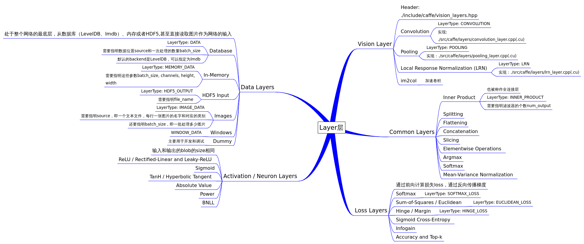
在Layer的派生类中,主要可以分为

(1)Vision Layers
Vison 层主要用于处理视觉图像相关的层,以图像作为输入,产生其他的图像。其主要特点是具有空间结构。
包含Convolution(conv_layer.hpp)、Pooling(pooling_layer.hpp)、Local Response Normalization(LRN)(lrn_layer.hpp)、im2col等,注:老版本的Caffe有头文件include/caffe/vision_layers.hpp,新版本中用include/caffe/layer/conv_layer.hpp等取代
(2)Loss Layers
这些层产生loss,如Softmax(SoftmaxWithLoss)、Sum-of-Squares / Euclidean(EuclideanLoss)、Hinge / Margin(HingeLoss)、Sigmoid Cross-Entropy(SigmoidCrossEntropyLoss)、Infogain(InfogainLoss)、Accuracy and Top-k等
(3)Activation / Neuron Layers
元素级别的运算,运算均为同址计算(in-place computation,返回值覆盖原值而占用新的内存)。如:ReLU / Rectified-Linear and Leaky-ReLU(ReLU)、Sigmoid(Sigmoid)、TanH / Hyperbolic Tangent(TanH)、Absolute Value(AbsVal)、Power(Power)、BNLL(BNLL)等
(4)Data Layers
网络的最底层,主要实现数据格式的转换,如:Database(Data)、In-Memory(MemoryData)、HDF5 Input(HDF5Data)、HDF5 Output(HDF5Output)、Images(ImageData)、Windows(WindowData)、Dummy(DummyData)等
(5)Common Layers
Caffe提供了单个层与多个层的连接。如:Inner Product(InnerProduct)、Splitting(Split)、Flattening(Flatten)、Reshape(Reshape)、Concatenation(Concat)、Slicing(Slice)、Elementwise(Eltwise)、Argmax(ArgMax)、Softmax(Softmax)、Mean-Variance Normalization(MVN)等
注,括号内为Layer Type,没有括号暂缺信息。
Net
1. 简介
一个Net由多个Layer组成。一个典型的网络从data layer(从磁盘中载入数据)出发到loss layer结束。
/**
 * @brief Connects Layer%s together into a directed acyclic graph (DAG)
 *        specified by a NetParameter.
 *
 * TODO(dox): more thorough description.
 */
template <typename Dtype>
class Net {
 public:
...
  /// @brief Initialize a network with a NetParameter.
  void Init(const NetParameter& param);
...

  const vector<Blob<Dtype>*>& Forward(const vector<Blob<Dtype>* > & bottom,
      Dtype* loss = NULL);
...
  /**
   * The network backward should take no input and output, since it solely
   * computes the gradient w.r.t the parameters, and the data has already been
   * provided during the forward pass.
   */
  void Backward();
  ...
  Dtype ForwardBackward(const vector<Blob<Dtype>* > & bottom) {
    Dtype loss;
    Forward(bottom, &loss);
    Backward();
    return loss;
  }
...

 protected:
  ...
  /// @brief The network name
  string name_;
  /// @brief The phase: TRAIN or TEST
  Phase phase_;
  /// @brief Individual layers in the net
  vector<shared_ptr<Layer<Dtype> > > layers_;
  /// @brief the blobs storing intermediate results between the layer.
  vector<shared_ptr<Blob<Dtype> > > blobs_;
  vector<vector<Blob<Dtype>*> > bottom_vecs_;
  vector<vector<Blob<Dtype>*> > top_vecs_;
  ...
  /// The root net that actually holds the shared layers in data parallelism
  const Net* const root_net_;
};
}  // namespace caffe
- 1
- 2
- 3
- 4
- 5
- 6
- 7
- 8
- 9
- 10
- 11
- 12
- 13
- 14
- 15
- 16
- 17
- 18
- 19
- 20
- 21
- 22
- 23
- 24
- 25
- 26
- 27
- 28
- 29
- 30
- 31
- 32
- 33
- 34
- 35
- 36
- 37
- 38
- 39
- 40
- 41
- 42
- 43
- 44
- 45
- 46
- 47
- 48
- 49
说明:
Init中,通过创建blob和layer搭建了整个网络框架,以及调用各层的SetUp函数。
blobs_存放这每一层产生的blobls的中间结果,bottom_vecs_存放每一层的bottom blobs,top_vecs_存放每一层的top blobs
Solver
1. 简介
其对网络进行求解,其作用有:
- 提供优化日志支持、创建用于学习的训练网络、创建用于评估的测试网络
- 通过调用forward / backward迭代地优化,更新权值
- 周期性地评估测试网络
- 通过优化了解model及solver的状态
2. 源代码
/**
 * @brief An interface for classes that perform optimization on Net%s.
 *
 * Requires implementation of ApplyUpdate to compute a parameter update
 * given the current state of the Net parameters.
 */
template <typename Dtype>
class Solver {
 public:
  explicit Solver(const SolverParameter& param,
      const Solver* root_solver = NULL);
  explicit Solver(const string& param_file, const Solver* root_solver = NULL);
  void Init(const SolverParameter& param);
  void InitTrainNet();
  void InitTestNets();
 ...
  // The main entry of the solver function. In default, iter will be zero. Pass
  // in a non-zero iter number to resume training for a pre-trained net.
  virtual void Solve(const char* resume_file = NULL);
  inline void Solve(const string resume_file) { Solve(resume_file.c_str()); }
  void Step(int iters);
...

 protected:
  // Make and apply the update value for the current iteration.
  virtual void ApplyUpdate() = 0;
  ...

  SolverParameter param_;
  int iter_;
  int current_step_;
  shared_ptr<Net<Dtype> > net_;
  vector<shared_ptr<Net<Dtype> > > test_nets_;
  vector<Callback*> callbacks_;
  vector<Dtype> losses_;
  Dtype smoothed_loss_;

  // The root solver that holds root nets (actually containing shared layers)
  // in data parallelism
  const Solver* const root_solver_;
...
};
- 1
- 2
- 3
- 4
- 5
- 6
- 7
- 8
- 9
- 10
- 11
- 12
- 13
- 14
- 15
- 16
- 17
- 18
- 19
- 20
- 21
- 22
- 23
- 24
- 25
- 26
- 27
- 28
- 29
- 30
- 31
- 32
- 33
- 34
- 35
- 36
- 37
- 38
- 39
- 40
- 41
- 42
说明:
shared_ptr<Net<Dtype>> net_为训练网络的指针,vector<shared_ptr<Net<Dtype>>> test_nets为测试网络的指针组,可见测试网络可以有多个- 一般来说训练网络跟测试网络在实现上会有区别,但是绝大部分网络层是相同的。
- 不同的模型训练方法通过重载函数ComputeUpdateValue( )实现计算update参数的核心功能
- caffe.cpp中的train( )函数训练模型,在这里实例化一个Solver对象,初始化后调用了Solver中的Solve( )方法。而这个Solve( )函数主要就是在迭代运行下面这两个函数。
- ComputeUpdateValue();
- net_->Update();
3. InitTrainNet
首先,ReadNetParamsFromTextFileOrDie(param_.net(), &net_param)把param_.net()(即examples/mnist/lenet_train_test.prototxt)中的信息读入net_param。
其次,net_.reset(new Net<Dtype>(net_param))重新构建网络,调用Net的构造方法。
然后,在构造方法中执行Net::init(),开始正式创建网络。其主要代码如下:
template <typename Dtype>
void Net<Dtype>::Init(const NetParameter& in_param) {
...
for (int layer_id = 0; layer_id < param.layer_size(); ++layer_id) {

  // Setup layer.
  const LayerParameter& layer_param = param.layer(layer_id);

  layers_.push_back(LayerRegistry<Dtype>::CreateLayer(layer_param));

  // Figure out this layer's input and output
  for (int bottom_id = 0; bottom_id < layer_param.bottom_size();  ++bottom_id) {
    const int blob_id = AppendBottom(param, layer_id, bottom_id, &available_blobs, &blob_name_to_idx);
    // If a blob needs backward, this layer should provide it.
    need_backward |= blob_need_backward_[blob_id];
  }
  int num_top = layer_param.top_size();
  for (int top_id = 0; top_id < num_top; ++top_id) {
    AppendTop(param, layer_id, top_id, &available_blobs, &blob_name_to_idx);
  }
...

layers_[layer_id]->SetUp(bottom_vecs_[layer_id], top_vecs_[layer_id]);
...
}

for (int param_id = 0; param_id < num_param_blobs; ++param_id) {
AppendParam(param, layer_id, param_id);
}

...
}
- 1
- 2
- 3
- 4
- 5
- 6
- 7
- 8
- 9
- 10
- 11
- 12
- 13
- 14
- 15
- 16
- 17
- 18
- 19
- 20
- 21
- 22
- 23
- 24
- 25
- 26
- 27
- 28
- 29
- 30
- 31
- 32
说明:
- Lenet5在caffe中共有5层,即
param.layer_size() == 5,以上代码每一次for循环创建一个网络层
每层网络是通过LayerRegistry::CreateLayer()创建的,类似与Solver的创建 - 14行
Net::AppendBottom(),对于layer_id这层,从Net::blob_中取出blob放入该层对应的bottom_vecs_[layer_id]中 - 20行
Net::AppendTop(),对于layer_id这层,创建blob(未包含数据)并放入Net::blob_中
Layer::SetUp() AppendParam中把每层网络的训练参数与网络变量learnable_params_绑定,在lenet中,只有conv1,conv2,ip1,ip2四层有参数,每层分别有参数与偏置参数两项参数,因而learnable_params_的size为8.
4. Solver的方法
- Stochastic Gradient Descent (type: “SGD”)
- AdaDelta (type: “AdaDelta”)
- Adaptive Gradient (type: “AdaGrad”)
- Adam (type: “Adam”)
- Nesterov’s Accelerated Gradient (type: “Nesterov”)
- RMSprop (type: “RMSProp”)
程序执行过程
训练网咯模型是由tools/caffe.cpp生成的工具caffe在模式train下完成的。
初始化过程总的来说,从main()、train()中创建Solver,在Solver中创建Net,在Net中创建Layer.
找到caffe.cpp的main函数中,通过GetBrewFunction(caffe::string(argv[1]))()调用执行train()函数。
train中,通过参数-examples/mnist/lenet_solver.prototxt把solver参数读入solver_param中。
随后注册并定义solver的指针(见第2节)
shared_ptr<caffe::Solver<float> >
solver(caffe::SolverRegistry<float>::CreateSolver(solver_param))
- 1
- 2
Solver的指针solver是通过SolverRegistry::CreateSolver创建的,CreateSolver函数中值得注意带是return registry[type](param)
  // Get a solver using a SolverParameter.
  static Solver<Dtype>* CreateSolver(const SolverParameter& param) {
    const string& type = param.type();
    CreatorRegistry& registry = Registry();
    CHECK_EQ(registry.count(type), 1) << "Unknown solver type: " << type
        << " (known types: " << SolverTypeListString() << ")";
    return registry[type](param);
  }
- 1
- 2
- 3
- 4
- 5
- 6
- 7
- 8
其中:
registry是一个map<string,Creator>: typedef std::map<string, Creator> CreatorRegistry
其中Creator是一个函数指针类型:typedef Solver<Dtype>* (*Creator)(const SolverParameter&)
registry[type]为一个函数指针变量,在Lenet5中,此处具体的值为 caffe::Creator_SGDSolver<float>(caffe::SolverParameter const&)
其中Creator_SGDSolver在以下宏中定义,
REGISTER_SOLVER_CLASS(SGD)
该宏完全展开得到的内容为:
template <typename Dtype>                                                    \
  Solver<Dtype>* Creator_SGDSolver(                                       \
      const SolverParameter& param)                                            \
  {                                                                            \
    return new SGDSolver<Dtype>(param);                                     \
  }                                                                            \
  static SolverRegisterer<float> g_creator_f_SGD("SGD", Creator_SGDSolver<float>);    \
  static SolverRegisterer<double> g_creator_d_SGD("SGD", Creator_SGDSolver<double>)
- 1
- 2
- 3
- 4
- 5
- 6
- 7
- 8
从上可以看出,registry[type](param)中实际上调用了SGDSolver的构造方法,事实上,网络是在SGDSolver的构造方法中初始化的。
SGDSolver的定义如下:
template <typename Dtype>
class SGDSolver : public Solver<Dtype> {
 public:
  explicit SGDSolver(const SolverParameter& param)
      : Solver<Dtype>(param) { PreSolve(); }
  explicit SGDSolver(const string& param_file)
      : Solver<Dtype>(param_file) { PreSolve(); }
......
- 1
- 2
- 3
- 4
- 5
- 6
- 7
- 8
SGDSolver继承与Solver<Dtype>,因而new SGDSolver<Dtype>(param)将执行Solver<Dtype>的构造函数,然后调用自身构造函数。整个网络带初始化即在这里面完成
Solver::Solve()函数
在这个函数里面,程序执行完网络的完整训练过程。
核心代码如下:
template <typename Dtype>
void Solver<Dtype>::Solve(const char* resume_file) {

  Step(param_.max_iter() - iter_);
  //..
    Snapshot();
  //..

  // some additional display
  // ...
}
- 1
- 2
- 3
- 4
- 5
- 6
- 7
- 8
- 9
- 10
- 11
说明:
值得关注的代码是Step(),在该函数中,进行了param_.max_iter()轮迭代(10000)
在Snapshot()中序列化model到文件
Solver::Step()函数
template <typename Dtype>
void Solver<Dtype>::Step(int iters) {

  //10000轮迭代
  while (iter_ < stop_iter) {

    // 每隔500轮进行一次测试
    if (param_.test_interval() && iter_ % param_.test_interval() == 0
        && (iter_ > 0 || param_.test_initialization())
        && Caffe::root_solver()) {
      // 测试网络,实际是执行前向传播计算loss
      TestAll();
    }

    // accumulate the loss and gradient
    Dtype loss = 0;
    for (int i = 0; i < param_.iter_size(); ++i) {
      // 执行反向传播,前向计算损失loss,并计算loss关于权值的偏导
      loss += net_->ForwardBackward(bottom_vec);
    }

    // 平滑loss,计算结果用于输出调试等
    loss /= param_.iter_size();
    // average the loss across iterations for smoothed reporting
    UpdateSmoothedLoss(loss, start_iter, average_loss);

    // 通过反向传播计算的偏导更新权值
    ApplyUpdate();

  }
}
- 1
- 2
- 3
- 4
- 5
- 6
- 7
- 8
- 9
- 10
- 11
- 12
- 13
- 14
- 15
- 16
- 17
- 18
- 19
- 20
- 21
- 22
- 23
- 24
- 25
- 26
- 27
- 28
- 29
- 30
- 31
Solver::TestAll()函数
在TestAll()中,调用Test(test_net_id)对每个测试网络test_net(不是训练网络train_net)进行测试。在Lenet中,只有一个测试网络,所以只调用一次Test(0)进行测试。
Test()函数里面做了两件事:
- 前向计算网络,得到网络损失.
- 通过测试网络的第11层accuracy层,与第12层loss层结果统计accuracy与loss信息。
Net::ForwardBackward()函数
Dtype ForwardBackward(const vector<Blob<Dtype>* > & bottom) {
    Dtype loss;
    Forward(bottom, &loss);
    Backward();
    return loss;
  }
- 1
- 2
- 3
- 4
- 5
- 6
说明:
- 前向计算。计算网络损失loss.
- 反向传播。计算loss关于网络权值的偏导.
Solver::ApplyUpdate()函数
根据反向传播阶段计算的loss关于网络权值的偏导,使用配置的学习策略,更新网络权值从而完成本轮学习。
训练完毕
至此,网络训练优化完成。在第3部分solve()函数中,最后对训练网络与测试网络再执行一轮额外的前行计算求得loss,以进行测试。
前向传播
对于ForwardFromTo有,对每层网络前向计算(start=0,end=11共12层网络)。
template <typename Dtype>
Dtype Net<Dtype>::ForwardFromTo(int start, int end) {

  for (int i = start; i <= end; ++i) {
    Dtype layer_loss = layers_[i]->Forward(bottom_vecs_[i], top_vecs_[i]);
    loss += layer_loss;
  }
  return loss;
}
- 1
- 2
- 3
- 4
- 5
- 6
- 7
- 8
- 9
在ForwardFromTo中,对网络的每层调用Forward函数,Forward中根据配置情况选择调用Forward_gpu还是Forward_cpu。
反向传播
Net::Backward()函数中调用BackwardFromTo函数,从网络最后一层到网络第一层反向调用每个网络层的Backward。
void Net<Dtype>::BackwardFromTo(int start, int end) {
  for (int i = start; i >= end; --i) {
    if (layer_need_backward_[i]) {
      layers_[i]->Backward(
          top_vecs_[i], bottom_need_backward_[i], bottom_vecs_[i]);
      if (debug_info_) { BackwardDebugInfo(i); }
    }
  }
}
- 1
- 2
- 3
- 4
- 5
- 6
- 7
- 8
- 9
权值更新
ApplyUpdate
void SGDSolver<Dtype>::ApplyUpdate() {
  // 获取该轮迭代的学习率(learning rate)
  Dtype rate = GetLearningRate();

  // 对每一层网络的权值进行更新
  // 在lenet中,只有`conv1`,`conv2`,`ip1`,`ip2`四层有参数
  // 每层分别有参数与偏置参数两项参数
  // 因而`learnable_params_`的size为8.
  for (int param_id = 0; param_id < this->net_->learnable_params().size();
       ++param_id) {
    // 归一化,iter_size为1不需要,因而lenet不需要
    Normalize(param_id);
    // 正则化
    Regularize(param_id);
    // 计算更新值\delta w
    ComputeUpdateValue(param_id, rate);
  }
  // 更新权值
  this->net_->Update();
}
- 1
- 2
- 3
- 4
- 5
- 6
- 7
- 8
- 9
- 10
- 11
- 12
- 13
- 14
- 15
- 16
- 17
- 18
- 19
- 20
学习速率的选择有
// The learning rate decay policy. The currently implemented learning rate
  // policies are as follows:
  //    - fixed: always return base_lr.
  //    - step: return base_lr * gamma ^ (floor(iter / step))
  //    - exp: return base_lr * gamma ^ iter
  //    - inv: return base_lr * (1 + gamma * iter) ^ (- power)
  //    - multistep: similar to step but it allows non uniform steps defined by
  //      stepvalue
  //    - poly: the effective learning rate follows a polynomial decay, to be
  //      zero by the max_iter. return base_lr (1 - iter/max_iter) ^ (power)
  //    - sigmoid: the effective learning rate follows a sigmod decay
  //      return base_lr ( 1/(1 + exp(-gamma * (iter - stepsize))))
  //
  // where base_lr, max_iter, gamma, step, stepvalue and power are defined
  // in the solver parameter protocol buffer, and iter is the current iteration.
- 1
- 2
- 3
- 4
- 5
- 6
- 7
- 8
- 9
- 10
- 11
- 12
- 13
- 14
- 15
Regularize
该函数实际执行以下公式
代码如下:
void SGDSolver<Dtype>::Regularize(int param_id) {
  const vector<Blob<Dtype>*>& net_params = this->net_->learnable_params();
  const vector<float>& net_params_weight_decay =
      this->net_->params_weight_decay();
  Dtype weight_decay = this->param_.weight_decay();
  string regularization_type = this->param_.regularization_type();
  // local_decay = 0.0005 in lenet
  Dtype local_decay = weight_decay * net_params_weight_decay[param_id];

  ...
      if (regularization_type == "L2") {
        // axpy means ax_plus_y. i.e., y = a*x + y
        caffe_axpy(net_params[param_id]->count(),
            local_decay,
            net_params[param_id]->cpu_data(),
            net_params[param_id]->mutable_cpu_diff());
      }
  ...
}
- 1
- 2
- 3
- 4
- 5
- 6
- 7
- 8
- 9
- 10
- 11
- 12
- 13
- 14
- 15
- 16
- 17
- 18
- 19
ComputeUpdateValue
该函数实际执行以下公式
代码如下:
void SGDSolver<Dtype>::ComputeUpdateValue(int param_id, Dtype rate) {
  const vector<Blob<Dtype>*>& net_params = this->net_->learnable_params();
  const vector<float>& net_params_lr = this->net_->params_lr();
  // momentum = 0.9 in lenet
  Dtype momentum = this->param_.momentum();
  // local_rate = lr_mult * global_rate
  // lr_mult为该层学习率乘子,在lenet_train_test.prototxt中设置
  Dtype local_rate = rate * net_params_lr[param_id];

  // Compute the update to history, then copy it to the parameter diff.

  ...
    // axpby means ax_plus_by. i.e., y = ax + by
    // 计算新的权值更新变化值 \delta w,结果保存在历史权值变化中
    caffe_cpu_axpby(net_params[param_id]->count(), local_rate,
              net_params[param_id]->cpu_diff(), momentum,
              history_[param_id]->mutable_cpu_data());

    // 从历史权值变化中把变化值 \delta w 保存到历史权值中diff中
    caffe_copy(net_params[param_id]->count(),
        history_[param_id]->cpu_data(),
        net_params[param_id]->mutable_cpu_diff());
   ...
}
- 1
- 2
- 3
- 4
- 5
- 6
- 7
- 8
- 9
- 10
- 11
- 12
- 13
- 14
- 15
- 16
- 17
- 18
- 19
- 20
- 21
- 22
- 23
- 24
net_->Update
实际执行以下公式:
caffe_axpy<Dtype>(count_, Dtype(-1),
        static_cast<const Dtype*>(diff_->cpu_data()),
        static_cast<Dtype*>(data_->mutable_cpu_data()));
- 1
- 2
- 3
- 4
Layer层的分析
(一) 数据层
数据的来源不同可以简单分为这么几种类型。官方的介绍
1. 数据来自于数据库(如LevelDB和LMDB)
层类型(layer type):Data
必须设置的参数:
- source: 包含数据库的目录名称,如examples/mnist/mnist_train_lmdb
- batch_size: 每次处理的数据个数,如64
可选的参数:
- rand_skip: 在开始的时候,路过某个数据的输入。通常对异步的SGD很有用。
- backend: 选择是采用LevelDB还是LMDB, 默认是LevelDB.
示例:
layer {
  name: "mnist" type: "Data" top: "data" top: "label" include { phase: TRAIN }
  transform_param {
    scale: 0.00390625 }
  data_param {
    source: "examples/mnist/mnist_train_lmdb" batch_size: 64 backend: LMDB }
}
- 1
- 2
- 3
- 4
- 5
- 6
- 7
- 8
- 9
- 10
- 11
- 12
- 13
- 14
- 15
- 16
- 17
2、数据来自于内存
层类型:MemoryData
必须设置的参数:
- batch_size:每一次处理的数据个数,比如2
- channels:通道数
- height:高度
- width: 宽度
示例:
layer {
  top: "data" top: "label" name: "memory_data" type: "MemoryData" memory_data_param{ batch_size: 2 height: 100 width: 100 channels: 1 }
  transform_param {
    scale: 0.0078125 mean_file: "mean.proto" mirror: false }
}
- 1
- 2
- 3
- 4
- 5
- 6
- 7
- 8
- 9
- 10
- 11
- 12
- 13
- 14
- 15
- 16
- 17
3、数据来自于HDF5
层类型:HDF5Data
必须设置的参数:
- source: 读取的文件名称
- batch_size: 每一次处理的数据个数
示例:
layer {
  name: "data" type: "HDF5Data" top: "data" top: "label" hdf5_data_param { source: "examples/hdf5_classification/data/train.txt" batch_size: 10 }
}
- 1
- 2
- 3
- 4
- 5
- 6
- 7
- 8
- 9
- 10
4、数据来自于图片
层类型:ImageData
必须设置的参数:
- source: 一个文本文件的名字,每一行给定一个图片文件的名称和标签(label)
- batch_size: 每一次处理的数据个数,即图片数
可选参数:
- rand_skip: 在开始的时候,路过某个数据的输入。通常对异步的SGD很有用。
- shuffle: 随机打乱顺序,默认值为false
- new_height,new_width: 如果设置,则将图片进行resize
示例:
layer {
  name: "data" type: "ImageData" top: "data" top: "label" transform_param { mirror: false crop_size: 227 mean_file: "data/ilsvrc12/imagenet_mean.binaryproto" }
  image_data_param {
    source: "examples/_temp/file_list.txt" batch_size: 50 new_height: 256 new_width: 256 }
}
- 1
- 2
- 3
- 4
- 5
- 6
- 7
- 8
- 9
- 10
- 11
- 12
- 13
- 14
- 15
- 16
- 17
5、数据来源于Windows
层类型:WindowData
必须设置的参数:
- source: 一个文本文件的名字
- batch_size: 每一次处理的数据个数,即图片数
示例:
layer {
  name: "data" type: "WindowData" top: "data" top: "label" include { phase: TRAIN }
  transform_param {
    mirror: true crop_size: 227 mean_file: "data/ilsvrc12/imagenet_mean.binaryproto" }
  window_data_param {
    source: "examples/finetune_pascal_detection/window_file_2007_trainval.txt" batch_size: 128 fg_threshold: 0.5 bg_threshold: 0.5 fg_fraction: 0.25 context_pad: 16 crop_mode: "warp" }
}
- 1
- 2
- 3
- 4
- 5
- 6
- 7
- 8
- 9
- 10
- 11
- 12
- 13
- 14
- 15
- 16
- 17
- 18
- 19
- 20
- 21
- 22
- 23
(二)视觉层
视觉层包括Convolution, Pooling, Local Response Normalization (LRN), im2col等层。
1、Convolution层:
就是卷积层,是卷积神经网络(CNN)的核心层。
层类型:Convolution
- lr_mult: 学习率的系数,最终的学习率是这个数乘以solver.prototxt配置文件中的base_lr。如果有两个lr_mult, 则第一个表示权值的学习率,第二个表示偏置项的学习率。一般偏置项的学习率是权值学习率的两倍。
在后面的convolution_param中,我们可以设定卷积层的特有参数。
必须设置的参数:
- num_output: 卷积核(filter)的个数
- kernel_size: 卷积核的大小。如果卷积核的长和宽不等,需要用kernel_h和kernel_w分别设定
其它参数: - stride: 卷积核的步长,默认为1。也可以用stride_h和stride_w来设置。
- pad: 扩充边缘,默认为0,不扩充。 扩充的时候是左右、上下对称的,比如卷积核的大小为5*5,那么pad设置为2,则四个边缘都扩充2个像素,即宽度和高度都扩充了4个像素,这样卷积运算之后的特征图就不会变小。也可以通过pad_h和pad_w来分别设定。
- weight_filler: 权值初始化。 默认为“constant”,值全为0,很多时候我们用”xavier”算法来进行初始化,也可以设置为”gaussian”
- bias_filler: 偏置项的初始化。一般设置为”constant”,值全为0。
- bias_term: 是否开启偏置项,默认为true, 开启
- group: 分组,默认为1组。如果大于1,我们限制卷积的连接操作在一个子集内。如果我们根据图像的通道来分组,那么第i个输出分组只能与第i个输入分组进行连接。
输入:n*c0*w0*h0
输出:n*c1*w1*h1
其中,c1就是参数中的num_output,生成的特征图个数
w1=(w0+2*pad-kernel_size)/stride+1;
h1=(h0+2*pad-kernel_size)/stride+1;
如果设置stride为1,前后两次卷积部分存在重叠。如果设置pad=(kernel_size-1)/2,则运算后,宽度和高度不变。
示例:
layer {
  name: "conv1" type: "Convolution" bottom: "data" top: "conv1" param { lr_mult: 1 }
  param {
    lr_mult: 2 }
  convolution_param {
    num_output: 20 kernel_size: 5 stride: 1 weight_filler { type: "xavier" }
    bias_filler {
      type: "constant" }
  }
}
- 1
- 2
- 3
- 4
- 5
- 6
- 7
- 8
- 9
- 10
- 11
- 12
- 13
- 14
- 15
- 16
- 17
- 18
- 19
- 20
- 21
- 22
- 23
2、Pooling层
也叫池化层,为了减少运算量和数据维度而设置的一种层。
层类型:Pooling
必须设置的参数:
+ kernel_size: 池化的核大小。也可以用kernel_h和kernel_w分别设定。
其它参数:
+ pool: 池化方法,默认为MAX。目前可用的方法有MAX, AVE, 或STOCHASTIC
+ pad: 和卷积层的pad的一样,进行边缘扩充。默认为0
+ stride: 池化的步长,默认为1。一般我们设置为2,即不重叠(步长=窗口大小)。也可以用stride_h和stride_w来设置。
示例:
layer {
  name: "pool1" type: "Pooling" bottom: "conv1" top: "pool1" pooling_param { pool: MAX kernel_size: 3 stride: 2 }
}
- 1
- 2
- 3
- 4
- 5
- 6
- 7
- 8
- 9
- 10
- 11
pooling层的运算方法基本是和卷积层是一样的。
输入:n*c*w0*h0
输出:n*c*w1*h1
和卷积层的区别就是其中的c保持不变
w1=(w0+2*pad-kernel_size)/stride+1;
h1=(h0+2*pad-kernel_size)/stride+1;
如果设置stride为2,前后两次卷积部分重叠。
3、Local Response Normalization (LRN)层
此层是对一个输入的局部区域进行归一化,达到“侧抑制”的效果。可去搜索AlexNet或GoogLenet,里面就用到了这个功能
层类型:LRN
参数:全部为可选,没有必须
- local_size: 默认为5。如果是跨通道LRN,则表示求和的通道数;如果是在通道内LRN,则表示求和的正方形区域长度。
- alpha: 默认为1,归一化公式中的参数。
- beta: 默认为5,归一化公式中的参数。
- norm_region: 默认为ACROSS_CHANNELS。有两个选择,ACROSS_CHANNELS表示在相邻的通道间求和归一化。WITHIN_CHANNEL表示在一个通道内部特定的区域内进行求和归一化。与前面的local_size参数对应。
归一化公式:对于每一个输入, 去除以,得到归一化后的输出
示例:
layers {
  name: "norm1" type: LRN bottom: "pool1" top: "norm1" lrn_param { local_size: 5 alpha: 0.0001 beta: 0.75 }
}
- 1
- 2
- 3
- 4
- 5
- 6
- 7
- 8
- 9
- 10
- 11
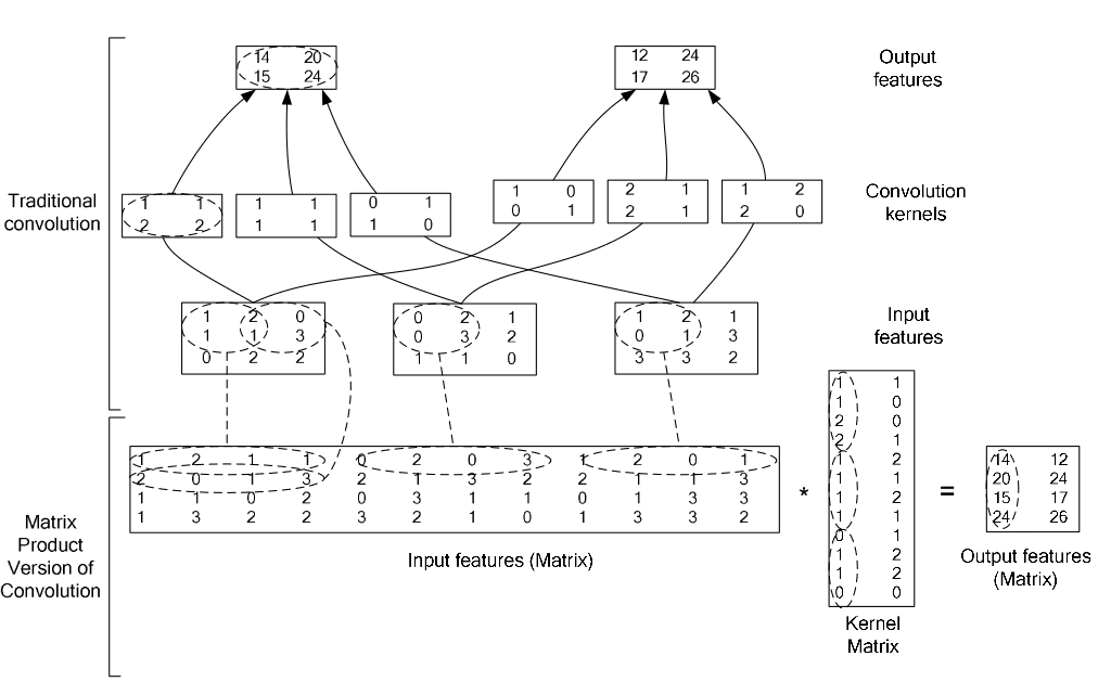
4、im2col层
如果对matlab比较熟悉的话,就应该知道im2col是什么意思。它先将一个大矩阵,重叠地划分为多个子矩阵,对每个子矩阵序列化成向量,最后得到另外一个矩阵。
看一看图就知道了:
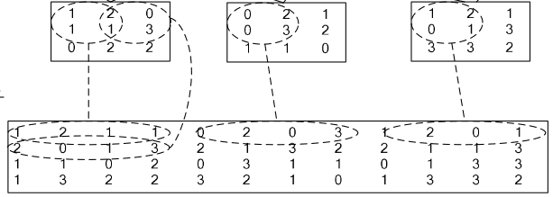
在caffe中,卷积运算就是先对数据进行im2col操作,再进行内积运算(inner product)。这样做,比原始的卷积操作速度更快。
看看两种卷积操作的异同:
(三)激活层
在激活层中,对输入数据进行激活操作(实际上就是一种函数变换),是逐元素进行运算的。从bottom得到一个blob数据输入,运算后,从top输入一个blob数据。在运算过程中,没有改变数据的大小,即输入和输出的数据大小是相等的。
输入:n*c*h*w
输出:n*c*h*w
常用的激活函数有sigmoid, tanh,relu等,下面分别介绍。
1、Sigmoid
对每个输入数据,利用sigmoid函数执行操作。这种层设置比较简单,没有额外的参数。
层类型:Sigmoid
示例:
layer {
  name: "encode1neuron" bottom: "encode1" top: "encode1neuron" type: "Sigmoid" }
- 1
- 2
- 3
- 4
- 5
- 6
2、ReLU / Rectified-Linear and Leaky-ReLU
ReLU是目前使用最多的激活函数,主要因为其收敛更快,并且能保持同样效果。
标准的ReLU函数为max(x, 0),当x>0时,输出x; 当x<=0时,输出0
f(x)=max(x,0)
层类型:ReLU
可选参数:
- negative_slope:默认为0. 对标准的ReLU函数进行变化,如果设置了这个值,那么数据为负数时,就不再设置为0,而是用原始数据乘以negative_slope
layer {
  name: "relu1" type: "ReLU" bottom: "pool1" top: "pool1" }
- 1
- 2
- 3
- 4
- 5
- 6
RELU层支持in-place计算,这意味着bottom的输出和输入相同以避免内存的消耗。
3、TanH / Hyperbolic Tangent
利用双曲正切函数对数据进行变换。
层类型:TanH
layer {
  name: "layer" bottom: "in" top: "out" type: "TanH" }
- 1
- 2
- 3
- 4
- 5
- 6
4、Absolute Value
求每个输入数据的绝对值。
f(x)=Abs(x)
层类型:AbsVal
layer {
  name: "layer" bottom: "in" top: "out" type: "AbsVal" }
- 1
- 2
- 3
- 4
- 5
- 6
5、Power
对每个输入数据进行幂运算
f(x)= (shift + scale * x) ^ power
层类型:Power
可选参数:
- power: 默认为1
- scale: 默认为1
- shift: 默认为0
layer {
  name: "layer" bottom: "in" top: "out" type: "Power" power_param { power: 2 scale: 1 shift: 0 }
}
- 1
- 2
- 3
- 4
- 5
- 6
- 7
- 8
- 9
- 10
- 11
6、BNLL
binomial normal log likelihood的简称
f(x)=log(1 + exp(x))
层类型:BNLL
layer {
  name: "layer" bottom: "in" top: "out" type: “BNLL” }
- 1
- 2
- 3
- 4
- 5
- 6
(四)常用层
包括:softmax_loss层,Inner Product层,accuracy层,reshape层和dropout层及其它们的参数配置。
1、softmax-loss
softmax-loss层和softmax层计算大致是相同的。softmax是一个分类器,计算的是类别的概率(Likelihood),是Logistic Regression 的一种推广。Logistic Regression 只能用于二分类,而softmax可以用于多分类。
softmax与softmax-loss的区别:
softmax计算公式:
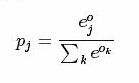
而softmax-loss计算公式:

关于两者的区别更加具体的介绍,可参考:softmax vs. softmax-loss
用户可能最终目的就是得到各个类别的概率似然值,这个时候就只需要一个 Softmax层,而不一定要进行softmax-Loss 操作;或者是用户有通过其他什么方式已经得到了某种概率似然值,然后要做最大似然估计,此时则只需要后面的 softmax-Loss 而不需要前面的 Softmax 操作。因此提供两个不同的 Layer 结构比只提供一个合在一起的 Softmax-Loss Layer 要灵活许多。
不管是softmax layer还是softmax-loss layer,都是没有参数的,只是层类型不同而也
softmax-loss layer:输出loss值
layer {
  name: "loss" type: "SoftmaxWithLoss" bottom: "ip1" bottom: "label" top: "loss" }
- 1
- 2
- 3
- 4
- 5
- 6
- 7
softmax layer: 输出似然值
layers {
  bottom: "cls3_fc"
  top: "prob"
  name: "prob"
  type: “Softmax"
}
- 1
- 2
- 3
- 4
- 5
- 6
2、Inner Product
全连接层,把输入当作成一个向量,输出也是一个简单向量(把输入数据blobs的width和height全变为1)。
输入: n*c0*h*w
输出: n*c1*1*1
全连接层实际上也是一种卷积层,只是它的卷积核大小和原数据大小一致。因此它的参数基本和卷积层的参数一样。
层类型:InnerProduct
lr_mult: 学习率的系数,最终的学习率是这个数乘以solver.prototxt配置文件中的base_lr。如果有两个lr_mult, 则第一个表示权值的学习率,第二个表示偏置项的学习率。一般偏置项的学习率是权值学习率的两倍。
必须设置的参数:
+ num_output: 过滤器(filfter)的个数
其它参数:
- weight_filler: 权值初始化。 默认为“constant”,值全为0,很多时候我们用”xavier”算法来进行初始化,也可以设置为”gaussian”
- bias_filler: 偏置项的初始化。一般设置为”constant”,值全为0。
- bias_term: 是否开启偏置项,默认为true, 开启
layer {
  name: "ip1" type: "InnerProduct" bottom: "pool2" top: "ip1" param { lr_mult: 1 }
  param {
    lr_mult: 2 }
  inner_product_param {
    num_output: 500 weight_filler { type: "xavier" }
    bias_filler {
      type: "constant" }
  }
}
- 1
- 2
- 3
- 4
- 5
- 6
- 7
- 8
- 9
- 10
- 11
- 12
- 13
- 14
- 15
- 16
- 17
- 18
- 19
- 20
- 21
3、accuracy
输出分类(预测)精确度,只有test阶段才有,因此需要加入include参数。
层类型:Accuracy
layer {
  name: "accuracy" type: "Accuracy" bottom: "ip2" bottom: "label" top: "accuracy" include { phase: TEST }
}
- 1
- 2
- 3
- 4
- 5
- 6
- 7
- 8
- 9
- 10
4、reshape
在不改变数据的情况下,改变输入的维度。
层类型:Reshape
先来看例子
layer {
    name: "reshape"
    type: "Reshape"
    bottom: "input"
    top: "output"
    reshape_param {
      shape {
        dim: 0  # copy the dimension from below
        dim: 2
        dim: 3
        dim: -1 # infer it from the other dimensions
      }
    }
  }
- 1
- 2
- 3
- 4
- 5
- 6
- 7
- 8
- 9
- 10
- 11
- 12
- 13
- 14
有一个可选的参数组shape, 用于指定blob数据的各维的值(blob是一个四维的数据:n*c*w*h)。
dim:0 表示维度不变,即输入和输出是相同的维度。
dim:2 或 dim:3 将原来的维度变成2或3
dim:-1 表示由系统自动计算维度。数据的总量不变,系统会根据blob数据的其它三维来自动计算当前维的维度值 。
假设原数据为:64*3*28*28, 表示64张3通道的28*28的彩色图片
经过reshape变换:
reshape_param {
      shape {
        dim: 0
        dim: 0
        dim: 14
        dim: -1
      }
    }
- 1
- 2
- 3
- 4
- 5
- 6
- 7
- 8
输出数据为:64*3*14*56
5、Dropout
Dropout是一个防止过拟合的trick。可以随机让网络某些隐含层节点的权重不工作。
先看例子:
layer {
  name: "drop7" type: "Dropout" bottom: "fc7-conv" top: "fc7-conv" dropout_param { dropout_ratio: 0.5 }
}layer {
  name: "drop7" type: "Dropout" bottom: "fc7-conv" top: "fc7-conv" dropout_param { dropout_ratio: 0.5 }
}
- 1
- 2
- 3
- 4
- 5
- 6
- 7
- 8
- 9
- 10
- 11
- 12
- 13
- 14
- 15
- 16
- 17
只需要设置一个dropout_ratio就可以了。
多线程
GPU
其他
Filter
Filter类在Caffe中用来初始化权值大小,有如下表的类型:
| 类型 | 派生类 | 说明 |
|---|---|---|
| constant | ConstantFiller | 使用一个常数(默认为0)初始化权值 |
| gaussian | GaussianFiller | 使用高斯分布初始化权值 |
| positive_unitball | PositiveUnitballFiller | |
| uniform | UniformFiller | 使用均为分布初始化权值 |
| xavier | XavierFiller | 使用xavier算法初始化权值 |
| msra | MSRAFiller | |
| bilinear | BilinearFiller |
其中, xavier 使用分布 x∼U(−3/n,+3/n)” role=”presentation” style=”position: relative;”>x∼U(−3/n−−−√,+3/n−−−√)x∼U(−3/n,+3/n)初始化权值w 为。总的来说n的值为输入输出规模相关,公式如下:
结构分析
caffe分为
1. Solver
2. Net
3. Layer
4. Blob
四层结构.
Solver : 负责模型的求解
Net : 负责定义网络的结构
Layer: 负责每一层网络功能的具体实现
Blob : 则定义数据,负责数据在每一层之间的流动。
Blob
1. 简介
Blob是:
- 对处理数据的一层封装,用于在Caffe中通信传递。
- 也为CPU和GPU间提供同步能力
- 数学上,是一个N维的C风格的存储数组
- 总的来说,Caffe使用Blob来交流数据,其是Caffe中标准的数组与统一的内存接口,它是多功能的,在不同的应用场景具有不同的含义,如可以是:batches of images(图像), model parameters(模型参数), and derivatives for optimization(最优化的导数)等。
2. 源代码
/**
 * @brief A wrapper around SyncedMemory holders serving as the basic
 *        computational unit through which Layer%s, Net%s, and Solver%s
 *        interact.
 *
 * TODO(dox): more thorough description.
 */
template <typename Dtype>
class Blob {
 public:
  Blob()
       : data_(), diff_(), count_(0), capacity_(0) {}

  /// @brief Deprecated; use <code>Blob(const vector<int>& shape)</code>.
  explicit Blob(const int num, const int channels, const int height,
      const int width);
  explicit Blob(const vector<int>& shape);

  .....

 protected:
  shared_ptr<SyncedMemory> data_;
  shared_ptr<SyncedMemory> diff_;
  shared_ptr<SyncedMemory> shape_data_;
  vector<int> shape_;
  int count_;
  int capacity_;

  DISABLE_COPY_AND_ASSIGN(Blob);
};  // class Blob
- 1
- 2
- 3
- 4
- 5
- 6
- 7
- 8
- 9
- 10
- 11
- 12
- 13
- 14
- 15
- 16
- 17
- 18
- 19
- 20
- 21
- 22
- 23
- 24
- 25
- 26
- 27
- 28
- 29
- 30
注:此处只保留了构造函数与成员变量。
说明:
- Blob在实现上是对SyncedMemory进行了一层封装。
- shape_为blob维度。
- data_为原始数据。
- diff_为梯度信息。
- count为该blob的总容量(即数据的size),函数
count(x,y)(或count(x))返回某个切片[x,y]([x,end])内容量,本质上就是shape[x]shape[x+1]....*shape[y]的值
3. Blob的shape
由源代码中可以注意到Blob有个成员变量:vector<ini> shape_
其作用:
- 对于图像数据,shape可以定义为4维的数组(Num, Channels, Height, Width)或(n, k, h, w),所以Blob数据维度为nkhw,Blob是row-major保存的,因此在(n, k, h, w)位置的值物理位置为((n K + k) H + h) W + w。其中Number是数据的batch size,对于256张图片为一个training batch的ImageNet来说n = 256;Channel是特征维度,如RGB图像k = 3
- 对于全连接网络,使用2D blobs (shape (N, D)),然后调用InnerProductLayer
- 对于参数,维度根据该层的类型和配置来确定。对于有3个输入96个输出的卷积层,Filter核 11 x 11,则blob为96 x 3 x 11 x 11. 对于全连接层,1000个输出,1024个输入,则blob为1000 x 1024.
4. SyncedMemory
由2知,Blob本质是对SyncedMemory的再封装。其核心代码如下:
/**
 * @brief Manages memory allocation and synchronization between the host (CPU)
 *        and device (GPU).
 *
 * TODO(dox): more thorough description.
 */
class SyncedMemory {
 public:
...
 const void* cpu_data();
 const void* gpu_data();
 void* mutable_cpu_data();
 void* mutable_gpu_data();
...
 private:
...
  void* cpu_ptr_;
  void* gpu_ptr_;
...
};  // class SyncedMemory
- 1
- 2
- 3
- 4
- 5
- 6
- 7
- 8
- 9
- 10
- 11
- 12
- 13
- 14
- 15
- 16
- 17
- 18
- 19
- 20
Blob同时保存了data_和diff_,其类型为SyncedMemory的指针。
对于data_(diff_相同),其实际值要么存储在CPU(cpu_ptr_)要么存储在GPU(gpu_ptr_),有两种方式访问CPU数据(GPU相同):
- 常量方式,
void* cpu_data(),其不改变cpu_ptr_指向存储区域的值。 - 可变方式,
void* mutable_cpu_data(),其可改变cpu_ptr_指向存储区值。
Layer
1. 简介
Layer是Caffe的基础以及基本计算单元。Caffe十分强调网络的层次性,可以说,一个网络的大部分功能都是以Layer的形式去展开的,如convolute,pooling,loss等等。
在创建一个Caffe模型的时候,也是以Layer为基础进行的,需按照src/caffe/proto/caffe.proto中定义的网络及参数格式定义网络 prototxt文件.
Layer的输入和输出就是Blob的数据。
每一层定义了三种操作
- Setup:Layer的初始化
- Forward:前向传导计算,根据bottom计算top,调用了Forward_cpu(必须实现)和Forward_gpu(可选,若未实现,则调用cpu的)
- Backward:反向传导计算,根据top计算bottom的梯度,其他同上
2.派生类分类
在Layer的派生类中,主要可以分为
(1)Vision Layers
Vison 层主要用于处理视觉图像相关的层,以图像作为输入,产生其他的图像。其主要特点是具有空间结构。
包含Convolution(conv_layer.hpp)、Pooling(pooling_layer.hpp)、Local Response Normalization(LRN)(lrn_layer.hpp)、im2col等,注:老版本的Caffe有头文件include/caffe/vision_layers.hpp,新版本中用include/caffe/layer/conv_layer.hpp等取代
(2)Loss Layers
这些层产生loss,如Softmax(SoftmaxWithLoss)、Sum-of-Squares / Euclidean(EuclideanLoss)、Hinge / Margin(HingeLoss)、Sigmoid Cross-Entropy(SigmoidCrossEntropyLoss)、Infogain(InfogainLoss)、Accuracy and Top-k等
(3)Activation / Neuron Layers
元素级别的运算,运算均为同址计算(in-place computation,返回值覆盖原值而占用新的内存)。如:ReLU / Rectified-Linear and Leaky-ReLU(ReLU)、Sigmoid(Sigmoid)、TanH / Hyperbolic Tangent(TanH)、Absolute Value(AbsVal)、Power(Power)、BNLL(BNLL)等
(4)Data Layers
网络的最底层,主要实现数据格式的转换,如:Database(Data)、In-Memory(MemoryData)、HDF5 Input(HDF5Data)、HDF5 Output(HDF5Output)、Images(ImageData)、Windows(WindowData)、Dummy(DummyData)等
(5)Common Layers
Caffe提供了单个层与多个层的连接。如:Inner Product(InnerProduct)、Splitting(Split)、Flattening(Flatten)、Reshape(Reshape)、Concatenation(Concat)、Slicing(Slice)、Elementwise(Eltwise)、Argmax(ArgMax)、Softmax(Softmax)、Mean-Variance Normalization(MVN)等
注,括号内为Layer Type,没有括号暂缺信息。
Net
1. 简介
一个Net由多个Layer组成。一个典型的网络从data layer(从磁盘中载入数据)出发到loss layer结束。
/**
 * @brief Connects Layer%s together into a directed acyclic graph (DAG)
 *        specified by a NetParameter.
 *
 * TODO(dox): more thorough description.
 */
template <typename Dtype>
class Net {
 public:
...
  /// @brief Initialize a network with a NetParameter.
  void Init(const NetParameter& param);
...

  const vector<Blob<Dtype>*>& Forward(const vector<Blob<Dtype>* > & bottom,
      Dtype* loss = NULL);
...
  /**
   * The network backward should take no input and output, since it solely
   * computes the gradient w.r.t the parameters, and the data has already been
   * provided during the forward pass.
   */
  void Backward();
  ...
  Dtype ForwardBackward(const vector<Blob<Dtype>* > & bottom) {
    Dtype loss;
    Forward(bottom, &loss);
    Backward();
    return loss;
  }
...

 protected:
  ...
  /// @brief The network name
  string name_;
  /// @brief The phase: TRAIN or TEST
  Phase phase_;
  /// @brief Individual layers in the net
  vector<shared_ptr<Layer<Dtype> > > layers_;
  /// @brief the blobs storing intermediate results between the layer.
  vector<shared_ptr<Blob<Dtype> > > blobs_;
  vector<vector<Blob<Dtype>*> > bottom_vecs_;
  vector<vector<Blob<Dtype>*> > top_vecs_;
  ...
  /// The root net that actually holds the shared layers in data parallelism
  const Net* const root_net_;
};
}  // namespace caffe
- 1
- 2
- 3
- 4
- 5
- 6
- 7
- 8
- 9
- 10
- 11
- 12
- 13
- 14
- 15
- 16
- 17
- 18
- 19
- 20
- 21
- 22
- 23
- 24
- 25
- 26
- 27
- 28
- 29
- 30
- 31
- 32
- 33
- 34
- 35
- 36
- 37
- 38
- 39
- 40
- 41
- 42
- 43
- 44
- 45
- 46
- 47
- 48
- 49
说明:
Init中,通过创建blob和layer搭建了整个网络框架,以及调用各层的SetUp函数。
blobs_存放这每一层产生的blobls的中间结果,bottom_vecs_存放每一层的bottom blobs,top_vecs_存放每一层的top blobs
Solver
1. 简介
其对网络进行求解,其作用有:
- 提供优化日志支持、创建用于学习的训练网络、创建用于评估的测试网络
- 通过调用forward / backward迭代地优化,更新权值
- 周期性地评估测试网络
- 通过优化了解model及solver的状态
2. 源代码
/**
 * @brief An interface for classes that perform optimization on Net%s.
 *
 * Requires implementation of ApplyUpdate to compute a parameter update
 * given the current state of the Net parameters.
 */
template <typename Dtype>
class Solver {
 public:
  explicit Solver(const SolverParameter& param,
      const Solver* root_solver = NULL);
  explicit Solver(const string& param_file, const Solver* root_solver = NULL);
  void Init(const SolverParameter& param);
  void InitTrainNet();
  void InitTestNets();
 ...
  // The main entry of the solver function. In default, iter will be zero. Pass
  // in a non-zero iter number to resume training for a pre-trained net.
  virtual void Solve(const char* resume_file = NULL);
  inline void Solve(const string resume_file) { Solve(resume_file.c_str()); }
  void Step(int iters);
...

 protected:
  // Make and apply the update value for the current iteration.
  virtual void ApplyUpdate() = 0;
  ...

  SolverParameter param_;
  int iter_;
  int current_step_;
  shared_ptr<Net<Dtype> > net_;
  vector<shared_ptr<Net<Dtype> > > test_nets_;
  vector<Callback*> callbacks_;
  vector<Dtype> losses_;
  Dtype smoothed_loss_;

  // The root solver that holds root nets (actually containing shared layers)
  // in data parallelism
  const Solver* const root_solver_;
...
};
- 1
- 2
- 3
- 4
- 5
- 6
- 7
- 8
- 9
- 10
- 11
- 12
- 13
- 14
- 15
- 16
- 17
- 18
- 19
- 20
- 21
- 22
- 23
- 24
- 25
- 26
- 27
- 28
- 29
- 30
- 31
- 32
- 33
- 34
- 35
- 36
- 37
- 38
- 39
- 40
- 41
- 42
说明:
shared_ptr<Net<Dtype>> net_为训练网络的指针,vector<shared_ptr<Net<Dtype>>> test_nets为测试网络的指针组,可见测试网络可以有多个- 一般来说训练网络跟测试网络在实现上会有区别,但是绝大部分网络层是相同的。
- 不同的模型训练方法通过重载函数ComputeUpdateValue( )实现计算update参数的核心功能
- caffe.cpp中的train( )函数训练模型,在这里实例化一个Solver对象,初始化后调用了Solver中的Solve( )方法。而这个Solve( )函数主要就是在迭代运行下面这两个函数。
- ComputeUpdateValue();
- net_->Update();
3. InitTrainNet
首先,ReadNetParamsFromTextFileOrDie(param_.net(), &net_param)把param_.net()(即examples/mnist/lenet_train_test.prototxt)中的信息读入net_param。
其次,net_.reset(new Net<Dtype>(net_param))重新构建网络,调用Net的构造方法。
然后,在构造方法中执行Net::init(),开始正式创建网络。其主要代码如下:
template <typename Dtype>
void Net<Dtype>::Init(const NetParameter& in_param) {
...
for (int layer_id = 0; layer_id < param.layer_size(); ++layer_id) {

  // Setup layer.
  const LayerParameter& layer_param = param.layer(layer_id);

  layers_.push_back(LayerRegistry<Dtype>::CreateLayer(layer_param));

  // Figure out this layer's input and output
  for (int bottom_id = 0; bottom_id < layer_param.bottom_size();  ++bottom_id) {
    const int blob_id = AppendBottom(param, layer_id, bottom_id, &available_blobs, &blob_name_to_idx);
    // If a blob needs backward, this layer should provide it.
    need_backward |= blob_need_backward_[blob_id];
  }
  int num_top = layer_param.top_size();
  for (int top_id = 0; top_id < num_top; ++top_id) {
    AppendTop(param, layer_id, top_id, &available_blobs, &blob_name_to_idx);
  }
...

layers_[layer_id]->SetUp(bottom_vecs_[layer_id], top_vecs_[layer_id]);
...
}

for (int param_id = 0; param_id < num_param_blobs; ++param_id) {
AppendParam(param, layer_id, param_id);
}

...
}
- 1
- 2
- 3
- 4
- 5
- 6
- 7
- 8
- 9
- 10
- 11
- 12
- 13
- 14
- 15
- 16
- 17
- 18
- 19
- 20
- 21
- 22
- 23
- 24
- 25
- 26
- 27
- 28
- 29
- 30
- 31
- 32
说明:
- Lenet5在caffe中共有5层,即
param.layer_size() == 5,以上代码每一次for循环创建一个网络层
每层网络是通过LayerRegistry::CreateLayer()创建的,类似与Solver的创建 - 14行
Net::AppendBottom(),对于layer_id这层,从Net::blob_中取出blob放入该层对应的bottom_vecs_[layer_id]中 - 20行
Net::AppendTop(),对于layer_id这层,创建blob(未包含数据)并放入Net::blob_中
Layer::SetUp() AppendParam中把每层网络的训练参数与网络变量learnable_params_绑定,在lenet中,只有conv1,conv2,ip1,ip2四层有参数,每层分别有参数与偏置参数两项参数,因而learnable_params_的size为8.
4. Solver的方法
- Stochastic Gradient Descent (type: “SGD”)
- AdaDelta (type: “AdaDelta”)
- Adaptive Gradient (type: “AdaGrad”)
- Adam (type: “Adam”)
- Nesterov’s Accelerated Gradient (type: “Nesterov”)
- RMSprop (type: “RMSProp”)
程序执行过程
训练网咯模型是由tools/caffe.cpp生成的工具caffe在模式train下完成的。
初始化过程总的来说,从main()、train()中创建Solver,在Solver中创建Net,在Net中创建Layer.
找到caffe.cpp的main函数中,通过GetBrewFunction(caffe::string(argv[1]))()调用执行train()函数。
train中,通过参数-examples/mnist/lenet_solver.prototxt把solver参数读入solver_param中。
随后注册并定义solver的指针(见第2节)
shared_ptr<caffe::Solver<float> >
solver(caffe::SolverRegistry<float>::CreateSolver(solver_param))
- 1
- 2
Solver的指针solver是通过SolverRegistry::CreateSolver创建的,CreateSolver函数中值得注意带是return registry[type](param)
  // Get a solver using a SolverParameter.
  static Solver<Dtype>* CreateSolver(const SolverParameter& param) {
    const string& type = param.type();
    CreatorRegistry& registry = Registry();
    CHECK_EQ(registry.count(type), 1) << "Unknown solver type: " << type
        << " (known types: " << SolverTypeListString() << ")";
    return registry[type](param);
  }
- 1
- 2
- 3
- 4
- 5
- 6
- 7
- 8
其中:
registry是一个map<string,Creator>: typedef std::map<string, Creator> CreatorRegistry
其中Creator是一个函数指针类型:typedef Solver<Dtype>* (*Creator)(const SolverParameter&)
registry[type]为一个函数指针变量,在Lenet5中,此处具体的值为 caffe::Creator_SGDSolver<float>(caffe::SolverParameter const&)
其中Creator_SGDSolver在以下宏中定义,
REGISTER_SOLVER_CLASS(SGD)
该宏完全展开得到的内容为:
template <typename Dtype>                                                    \
  Solver<Dtype>* Creator_SGDSolver(                                       \
      const SolverParameter& param)                                            \
  {                                                                            \
    return new SGDSolver<Dtype>(param);                                     \
  }                                                                            \
  static SolverRegisterer<float> g_creator_f_SGD("SGD", Creator_SGDSolver<float>);    \
  static SolverRegisterer<double> g_creator_d_SGD("SGD", Creator_SGDSolver<double>)
- 1
- 2
- 3
- 4
- 5
- 6
- 7
- 8
从上可以看出,registry[type](param)中实际上调用了SGDSolver的构造方法,事实上,网络是在SGDSolver的构造方法中初始化的。
SGDSolver的定义如下:
template <typename Dtype>
class SGDSolver : public Solver<Dtype> {
 public:
  explicit SGDSolver(const SolverParameter& param)
      : Solver<Dtype>(param) { PreSolve(); }
  explicit SGDSolver(const string& param_file)
      : Solver<Dtype>(param_file) { PreSolve(); }
......
- 1
- 2
- 3
- 4
- 5
- 6
- 7
- 8
SGDSolver继承与Solver<Dtype>,因而new SGDSolver<Dtype>(param)将执行Solver<Dtype>的构造函数,然后调用自身构造函数。整个网络带初始化即在这里面完成
Solver::Solve()函数
在这个函数里面,程序执行完网络的完整训练过程。
核心代码如下:
template <typename Dtype>
void Solver<Dtype>::Solve(const char* resume_file) {

  Step(param_.max_iter() - iter_);
  //..
    Snapshot();
  //..

  // some additional display
  // ...
}
- 1
- 2
- 3
- 4
- 5
- 6
- 7
- 8
- 9
- 10
- 11
说明:
值得关注的代码是Step(),在该函数中,进行了param_.max_iter()轮迭代(10000)
在Snapshot()中序列化model到文件
Solver::Step()函数
template <typename Dtype>
void Solver<Dtype>::Step(int iters) {

  //10000轮迭代
  while (iter_ < stop_iter) {

    // 每隔500轮进行一次测试
    if (param_.test_interval() && iter_ % param_.test_interval() == 0
        && (iter_ > 0 || param_.test_initialization())
        && Caffe::root_solver()) {
      // 测试网络,实际是执行前向传播计算loss
      TestAll();
    }

    // accumulate the loss and gradient
    Dtype loss = 0;
    for (int i = 0; i < param_.iter_size(); ++i) {
      // 执行反向传播,前向计算损失loss,并计算loss关于权值的偏导
      loss += net_->ForwardBackward(bottom_vec);
    }

    // 平滑loss,计算结果用于输出调试等
    loss /= param_.iter_size();
    // average the loss across iterations for smoothed reporting
    UpdateSmoothedLoss(loss, start_iter, average_loss);

    // 通过反向传播计算的偏导更新权值
    ApplyUpdate();

  }
}
- 1
- 2
- 3
- 4
- 5
- 6
- 7
- 8
- 9
- 10
- 11
- 12
- 13
- 14
- 15
- 16
- 17
- 18
- 19
- 20
- 21
- 22
- 23
- 24
- 25
- 26
- 27
- 28
- 29
- 30
- 31
Solver::TestAll()函数
在TestAll()中,调用Test(test_net_id)对每个测试网络test_net(不是训练网络train_net)进行测试。在Lenet中,只有一个测试网络,所以只调用一次Test(0)进行测试。
Test()函数里面做了两件事:
- 前向计算网络,得到网络损失.
- 通过测试网络的第11层accuracy层,与第12层loss层结果统计accuracy与loss信息。
Net::ForwardBackward()函数
Dtype ForwardBackward(const vector<Blob<Dtype>* > & bottom) {
    Dtype loss;
    Forward(bottom, &loss);
    Backward();
    return loss;
  }
- 1
- 2
- 3
- 4
- 5
- 6
说明:
- 前向计算。计算网络损失loss.
- 反向传播。计算loss关于网络权值的偏导.
Solver::ApplyUpdate()函数
根据反向传播阶段计算的loss关于网络权值的偏导,使用配置的学习策略,更新网络权值从而完成本轮学习。
训练完毕
至此,网络训练优化完成。在第3部分solve()函数中,最后对训练网络与测试网络再执行一轮额外的前行计算求得loss,以进行测试。
前向传播
对于ForwardFromTo有,对每层网络前向计算(start=0,end=11共12层网络)。
template <typename Dtype>
Dtype Net<Dtype>::ForwardFromTo(int start, int end) {

  for (int i = start; i <= end; ++i) {
    Dtype layer_loss = layers_[i]->Forward(bottom_vecs_[i], top_vecs_[i]);
    loss += layer_loss;
  }
  return loss;
}
- 1
- 2
- 3
- 4
- 5
- 6
- 7
- 8
- 9
在ForwardFromTo中,对网络的每层调用Forward函数,Forward中根据配置情况选择调用Forward_gpu还是Forward_cpu。
反向传播
Net::Backward()函数中调用BackwardFromTo函数,从网络最后一层到网络第一层反向调用每个网络层的Backward。
void Net<Dtype>::BackwardFromTo(int start, int end) {
  for (int i = start; i >= end; --i) {
    if (layer_need_backward_[i]) {
      layers_[i]->Backward(
          top_vecs_[i], bottom_need_backward_[i], bottom_vecs_[i]);
      if (debug_info_) { BackwardDebugInfo(i); }
    }
  }
}
- 1
- 2
- 3
- 4
- 5
- 6
- 7
- 8
- 9
权值更新
ApplyUpdate
void SGDSolver<Dtype>::ApplyUpdate() {
  // 获取该轮迭代的学习率(learning rate)
  Dtype rate = GetLearningRate();

  // 对每一层网络的权值进行更新
  // 在lenet中,只有`conv1`,`conv2`,`ip1`,`ip2`四层有参数
  // 每层分别有参数与偏置参数两项参数
  // 因而`learnable_params_`的size为8.
  for (int param_id = 0; param_id < this->net_->learnable_params().size();
       ++param_id) {
    // 归一化,iter_size为1不需要,因而lenet不需要
    Normalize(param_id);
    // 正则化
    Regularize(param_id);
    // 计算更新值\delta w
    ComputeUpdateValue(param_id, rate);
  }
  // 更新权值
  this->net_->Update();
}
- 1
- 2
- 3
- 4
- 5
- 6
- 7
- 8
- 9
- 10
- 11
- 12
- 13
- 14
- 15
- 16
- 17
- 18
- 19
- 20
学习速率的选择有
// The learning rate decay policy. The currently implemented learning rate
  // policies are as follows:
  //    - fixed: always return base_lr.
  //    - step: return base_lr * gamma ^ (floor(iter / step))
  //    - exp: return base_lr * gamma ^ iter
  //    - inv: return base_lr * (1 + gamma * iter) ^ (- power)
  //    - multistep: similar to step but it allows non uniform steps defined by
  //      stepvalue
  //    - poly: the effective learning rate follows a polynomial decay, to be
  //      zero by the max_iter. return base_lr (1 - iter/max_iter) ^ (power)
  //    - sigmoid: the effective learning rate follows a sigmod decay
  //      return base_lr ( 1/(1 + exp(-gamma * (iter - stepsize))))
  //
  // where base_lr, max_iter, gamma, step, stepvalue and power are defined
  // in the solver parameter protocol buffer, and iter is the current iteration.
- 1
- 2
- 3
- 4
- 5
- 6
- 7
- 8
- 9
- 10
- 11
- 12
- 13
- 14
- 15
Regularize
该函数实际执行以下公式
代码如下:
void SGDSolver<Dtype>::Regularize(int param_id) {
  const vector<Blob<Dtype>*>& net_params = this->net_->learnable_params();
  const vector<float>& net_params_weight_decay =
      this->net_->params_weight_decay();
  Dtype weight_decay = this->param_.weight_decay();
  string regularization_type = this->param_.regularization_type();
  // local_decay = 0.0005 in lenet
  Dtype local_decay = weight_decay * net_params_weight_decay[param_id];

  ...
      if (regularization_type == "L2") {
        // axpy means ax_plus_y. i.e., y = a*x + y
        caffe_axpy(net_params[param_id]->count(),
            local_decay,
            net_params[param_id]->cpu_data(),
            net_params[param_id]->mutable_cpu_diff());
      }
  ...
}
- 1
- 2
- 3
- 4
- 5
- 6
- 7
- 8
- 9
- 10
- 11
- 12
- 13
- 14
- 15
- 16
- 17
- 18
- 19
ComputeUpdateValue
该函数实际执行以下公式
代码如下:
void SGDSolver<Dtype>::ComputeUpdateValue(int param_id, Dtype rate) {
  const vector<Blob<Dtype>*>& net_params = this->net_->learnable_params();
  const vector<float>& net_params_lr = this->net_->params_lr();
  // momentum = 0.9 in lenet
  Dtype momentum = this->param_.momentum();
  // local_rate = lr_mult * global_rate
  // lr_mult为该层学习率乘子,在lenet_train_test.prototxt中设置
  Dtype local_rate = rate * net_params_lr[param_id];

  // Compute the update to history, then copy it to the parameter diff.

  ...
    // axpby means ax_plus_by. i.e., y = ax + by
    // 计算新的权值更新变化值 \delta w,结果保存在历史权值变化中
    caffe_cpu_axpby(net_params[param_id]->count(), local_rate,
              net_params[param_id]->cpu_diff(), momentum,
              history_[param_id]->mutable_cpu_data());

    // 从历史权值变化中把变化值 \delta w 保存到历史权值中diff中
    caffe_copy(net_params[param_id]->count(),
        history_[param_id]->cpu_data(),
        net_params[param_id]->mutable_cpu_diff());
   ...
}
- 1
- 2
- 3
- 4
- 5
- 6
- 7
- 8
- 9
- 10
- 11
- 12
- 13
- 14
- 15
- 16
- 17
- 18
- 19
- 20
- 21
- 22
- 23
- 24
net_->Update
实际执行以下公式:
caffe_axpy<Dtype>(count_, Dtype(-1),
        static_cast<const Dtype*>(diff_->cpu_data()),
        static_cast<Dtype*>(data_->mutable_cpu_data()));
- 1
- 2
- 3
- 4
Layer层的分析
(一) 数据层
数据的来源不同可以简单分为这么几种类型。官方的介绍
1. 数据来自于数据库(如LevelDB和LMDB)
层类型(layer type):Data
必须设置的参数:
- source: 包含数据库的目录名称,如examples/mnist/mnist_train_lmdb
- batch_size: 每次处理的数据个数,如64
可选的参数:
- rand_skip: 在开始的时候,路过某个数据的输入。通常对异步的SGD很有用。
- backend: 选择是采用LevelDB还是LMDB, 默认是LevelDB.
示例:
layer {
  name: "mnist" type: "Data" top: "data" top: "label" include { phase: TRAIN }
  transform_param {
    scale: 0.00390625 }
  data_param {
    source: "examples/mnist/mnist_train_lmdb" batch_size: 64 backend: LMDB }
}
- 1
- 2
- 3
- 4
- 5
- 6
- 7
- 8
- 9
- 10
- 11
- 12
- 13
- 14
- 15
- 16
- 17
2、数据来自于内存
层类型:MemoryData
必须设置的参数:
- batch_size:每一次处理的数据个数,比如2
- channels:通道数
- height:高度
- width: 宽度
示例:
layer {
  top: "data" top: "label" name: "memory_data" type: "MemoryData" memory_data_param{ batch_size: 2 height: 100 width: 100 channels: 1 }
  transform_param {
    scale: 0.0078125 mean_file: "mean.proto" mirror: false }
}
- 1
- 2
- 3
- 4
- 5
- 6
- 7
- 8
- 9
- 10
- 11
- 12
- 13
- 14
- 15
- 16
- 17
3、数据来自于HDF5
层类型:HDF5Data
必须设置的参数:
- source: 读取的文件名称
- batch_size: 每一次处理的数据个数
示例:
layer {
  name: "data" type: "HDF5Data" top: "data" top: "label" hdf5_data_param { source: "examples/hdf5_classification/data/train.txt" batch_size: 10 }
}
- 1
- 2
- 3
- 4
- 5
- 6
- 7
- 8
- 9
- 10
4、数据来自于图片
层类型:ImageData
必须设置的参数:
- source: 一个文本文件的名字,每一行给定一个图片文件的名称和标签(label)
- batch_size: 每一次处理的数据个数,即图片数
可选参数:
- rand_skip: 在开始的时候,路过某个数据的输入。通常对异步的SGD很有用。
- shuffle: 随机打乱顺序,默认值为false
- new_height,new_width: 如果设置,则将图片进行resize
示例:
layer {
  name: "data" type: "ImageData" top: "data" top: "label" transform_param { mirror: false crop_size: 227 mean_file: "data/ilsvrc12/imagenet_mean.binaryproto" }
  image_data_param {
    source: "examples/_temp/file_list.txt" batch_size: 50 new_height: 256 new_width: 256 }
}
- 1
- 2
- 3
- 4
- 5
- 6
- 7
- 8
- 9
- 10
- 11
- 12
- 13
- 14
- 15
- 16
- 17
5、数据来源于Windows
层类型:WindowData
必须设置的参数:
- source: 一个文本文件的名字
- batch_size: 每一次处理的数据个数,即图片数
示例:
layer {
  name: "data" type: "WindowData" top: "data" top: "label" include { phase: TRAIN }
  transform_param {
    mirror: true crop_size: 227 mean_file: "data/ilsvrc12/imagenet_mean.binaryproto" }
  window_data_param {
    source: "examples/finetune_pascal_detection/window_file_2007_trainval.txt" batch_size: 128 fg_threshold: 0.5 bg_threshold: 0.5 fg_fraction: 0.25 context_pad: 16 crop_mode: "warp" }
}
- 1
- 2
- 3
- 4
- 5
- 6
- 7
- 8
- 9
- 10
- 11
- 12
- 13
- 14
- 15
- 16
- 17
- 18
- 19
- 20
- 21
- 22
- 23
(二)视觉层
视觉层包括Convolution, Pooling, Local Response Normalization (LRN), im2col等层。
1、Convolution层:
就是卷积层,是卷积神经网络(CNN)的核心层。
层类型:Convolution
- lr_mult: 学习率的系数,最终的学习率是这个数乘以solver.prototxt配置文件中的base_lr。如果有两个lr_mult, 则第一个表示权值的学习率,第二个表示偏置项的学习率。一般偏置项的学习率是权值学习率的两倍。
在后面的convolution_param中,我们可以设定卷积层的特有参数。
必须设置的参数:
- num_output: 卷积核(filter)的个数
- kernel_size: 卷积核的大小。如果卷积核的长和宽不等,需要用kernel_h和kernel_w分别设定
其它参数: - stride: 卷积核的步长,默认为1。也可以用stride_h和stride_w来设置。
- pad: 扩充边缘,默认为0,不扩充。 扩充的时候是左右、上下对称的,比如卷积核的大小为5*5,那么pad设置为2,则四个边缘都扩充2个像素,即宽度和高度都扩充了4个像素,这样卷积运算之后的特征图就不会变小。也可以通过pad_h和pad_w来分别设定。
- weight_filler: 权值初始化。 默认为“constant”,值全为0,很多时候我们用”xavier”算法来进行初始化,也可以设置为”gaussian”
- bias_filler: 偏置项的初始化。一般设置为”constant”,值全为0。
- bias_term: 是否开启偏置项,默认为true, 开启
- group: 分组,默认为1组。如果大于1,我们限制卷积的连接操作在一个子集内。如果我们根据图像的通道来分组,那么第i个输出分组只能与第i个输入分组进行连接。
输入:n*c0*w0*h0
输出:n*c1*w1*h1
其中,c1就是参数中的num_output,生成的特征图个数
w1=(w0+2*pad-kernel_size)/stride+1;
h1=(h0+2*pad-kernel_size)/stride+1;
如果设置stride为1,前后两次卷积部分存在重叠。如果设置pad=(kernel_size-1)/2,则运算后,宽度和高度不变。
示例:
layer {
  name: "conv1" type: "Convolution" bottom: "data" top: "conv1" param { lr_mult: 1 }
  param {
    lr_mult: 2 }
  convolution_param {
    num_output: 20 kernel_size: 5 stride: 1 weight_filler { type: "xavier" }
    bias_filler {
      type: "constant" }
  }
}
- 1
- 2
- 3
- 4
- 5
- 6
- 7
- 8
- 9
- 10
- 11
- 12
- 13
- 14
- 15
- 16
- 17
- 18
- 19
- 20
- 21
- 22
- 23
2、Pooling层
也叫池化层,为了减少运算量和数据维度而设置的一种层。
层类型:Pooling
必须设置的参数:
+ kernel_size: 池化的核大小。也可以用kernel_h和kernel_w分别设定。
其它参数:
+ pool: 池化方法,默认为MAX。目前可用的方法有MAX, AVE, 或STOCHASTIC
+ pad: 和卷积层的pad的一样,进行边缘扩充。默认为0
+ stride: 池化的步长,默认为1。一般我们设置为2,即不重叠(步长=窗口大小)。也可以用stride_h和stride_w来设置。
示例:
layer {
  name: "pool1" type: "Pooling" bottom: "conv1" top: "pool1" pooling_param { pool: MAX kernel_size: 3 stride: 2 }
}
- 1
- 2
- 3
- 4
- 5
- 6
- 7
- 8
- 9
- 10
- 11
pooling层的运算方法基本是和卷积层是一样的。
输入:n*c*w0*h0
输出:n*c*w1*h1
和卷积层的区别就是其中的c保持不变
w1=(w0+2*pad-kernel_size)/stride+1;
h1=(h0+2*pad-kernel_size)/stride+1;
如果设置stride为2,前后两次卷积部分重叠。
3、Local Response Normalization (LRN)层
此层是对一个输入的局部区域进行归一化,达到“侧抑制”的效果。可去搜索AlexNet或GoogLenet,里面就用到了这个功能
层类型:LRN
参数:全部为可选,没有必须
- local_size: 默认为5。如果是跨通道LRN,则表示求和的通道数;如果是在通道内LRN,则表示求和的正方形区域长度。
- alpha: 默认为1,归一化公式中的参数。
- beta: 默认为5,归一化公式中的参数。
- norm_region: 默认为ACROSS_CHANNELS。有两个选择,ACROSS_CHANNELS表示在相邻的通道间求和归一化。WITHIN_CHANNEL表示在一个通道内部特定的区域内进行求和归一化。与前面的local_size参数对应。
归一化公式:对于每一个输入, 去除以,得到归一化后的输出
示例:
layers {
  name: "norm1" type: LRN bottom: "pool1" top: "norm1" lrn_param { local_size: 5 alpha: 0.0001 beta: 0.75 }
}
- 1
- 2
- 3
- 4
- 5
- 6
- 7
- 8
- 9
- 10
- 11
4、im2col层
如果对matlab比较熟悉的话,就应该知道im2col是什么意思。它先将一个大矩阵,重叠地划分为多个子矩阵,对每个子矩阵序列化成向量,最后得到另外一个矩阵。
看一看图就知道了:
在caffe中,卷积运算就是先对数据进行im2col操作,再进行内积运算(inner product)。这样做,比原始的卷积操作速度更快。
看看两种卷积操作的异同:
(三)激活层
在激活层中,对输入数据进行激活操作(实际上就是一种函数变换),是逐元素进行运算的。从bottom得到一个blob数据输入,运算后,从top输入一个blob数据。在运算过程中,没有改变数据的大小,即输入和输出的数据大小是相等的。
输入:n*c*h*w
输出:n*c*h*w
常用的激活函数有sigmoid, tanh,relu等,下面分别介绍。
1、Sigmoid
对每个输入数据,利用sigmoid函数执行操作。这种层设置比较简单,没有额外的参数。
层类型:Sigmoid
示例:
layer {
  name: "encode1neuron" bottom: "encode1" top: "encode1neuron" type: "Sigmoid" }
- 1
- 2
- 3
- 4
- 5
- 6
2、ReLU / Rectified-Linear and Leaky-ReLU
ReLU是目前使用最多的激活函数,主要因为其收敛更快,并且能保持同样效果。
标准的ReLU函数为max(x, 0),当x>0时,输出x; 当x<=0时,输出0
f(x)=max(x,0)
层类型:ReLU
可选参数:
- negative_slope:默认为0. 对标准的ReLU函数进行变化,如果设置了这个值,那么数据为负数时,就不再设置为0,而是用原始数据乘以negative_slope
layer {
  name: "relu1" type: "ReLU" bottom: "pool1" top: "pool1" }
- 1
- 2
- 3
- 4
- 5
- 6
RELU层支持in-place计算,这意味着bottom的输出和输入相同以避免内存的消耗。
3、TanH / Hyperbolic Tangent
利用双曲正切函数对数据进行变换。
层类型:TanH
layer {
  name: "layer" bottom: "in" top: "out" type: "TanH" }
- 1
- 2
- 3
- 4
- 5
- 6
4、Absolute Value
求每个输入数据的绝对值。
f(x)=Abs(x)
层类型:AbsVal
layer {
  name: "layer" bottom: "in" top: "out" type: "AbsVal" }
- 1
- 2
- 3
- 4
- 5
- 6
5、Power
对每个输入数据进行幂运算
f(x)= (shift + scale * x) ^ power
层类型:Power
可选参数:
- power: 默认为1
- scale: 默认为1
- shift: 默认为0
layer {
  name: "layer" bottom: "in" top: "out" type: "Power" power_param { power: 2 scale: 1 shift: 0 }
}
- 1
- 2
- 3
- 4
- 5
- 6
- 7
- 8
- 9
- 10
- 11
6、BNLL
binomial normal log likelihood的简称
f(x)=log(1 + exp(x))
层类型:BNLL
layer {
  name: "layer" bottom: "in" top: "out" type: “BNLL” }
- 1
- 2
- 3
- 4
- 5
- 6
(四)常用层
包括:softmax_loss层,Inner Product层,accuracy层,reshape层和dropout层及其它们的参数配置。
1、softmax-loss
softmax-loss层和softmax层计算大致是相同的。softmax是一个分类器,计算的是类别的概率(Likelihood),是Logistic Regression 的一种推广。Logistic Regression 只能用于二分类,而softmax可以用于多分类。
softmax与softmax-loss的区别:
softmax计算公式:
而softmax-loss计算公式:
关于两者的区别更加具体的介绍,可参考:softmax vs. softmax-loss
用户可能最终目的就是得到各个类别的概率似然值,这个时候就只需要一个 Softmax层,而不一定要进行softmax-Loss 操作;或者是用户有通过其他什么方式已经得到了某种概率似然值,然后要做最大似然估计,此时则只需要后面的 softmax-Loss 而不需要前面的 Softmax 操作。因此提供两个不同的 Layer 结构比只提供一个合在一起的 Softmax-Loss Layer 要灵活许多。
不管是softmax layer还是softmax-loss layer,都是没有参数的,只是层类型不同而也
softmax-loss layer:输出loss值
layer {
  name: "loss" type: "SoftmaxWithLoss" bottom: "ip1" bottom: "label" top: "loss" }
- 1
- 2
- 3
- 4
- 5
- 6
- 7
softmax layer: 输出似然值
layers {
  bottom: "cls3_fc"
  top: "prob"
  name: "prob"
  type: “Softmax"
}
- 1
- 2
- 3
- 4
- 5
- 6
2、Inner Product
全连接层,把输入当作成一个向量,输出也是一个简单向量(把输入数据blobs的width和height全变为1)。
输入: n*c0*h*w
输出: n*c1*1*1
全连接层实际上也是一种卷积层,只是它的卷积核大小和原数据大小一致。因此它的参数基本和卷积层的参数一样。
层类型:InnerProduct
lr_mult: 学习率的系数,最终的学习率是这个数乘以solver.prototxt配置文件中的base_lr。如果有两个lr_mult, 则第一个表示权值的学习率,第二个表示偏置项的学习率。一般偏置项的学习率是权值学习率的两倍。
必须设置的参数:
+ num_output: 过滤器(filfter)的个数
其它参数:
- weight_filler: 权值初始化。 默认为“constant”,值全为0,很多时候我们用”xavier”算法来进行初始化,也可以设置为”gaussian”
- bias_filler: 偏置项的初始化。一般设置为”constant”,值全为0。
- bias_term: 是否开启偏置项,默认为true, 开启
layer {
  name: "ip1" type: "InnerProduct" bottom: "pool2" top: "ip1" param { lr_mult: 1 }
  param {
    lr_mult: 2 }
  inner_product_param {
    num_output: 500 weight_filler { type: "xavier" }
    bias_filler {
      type: "constant" }
  }
}
- 1
- 2
- 3
- 4
- 5
- 6
- 7
- 8
- 9
- 10
- 11
- 12
- 13
- 14
- 15
- 16
- 17
- 18
- 19
- 20
- 21
3、accuracy
输出分类(预测)精确度,只有test阶段才有,因此需要加入include参数。
层类型:Accuracy
layer {
  name: "accuracy" type: "Accuracy" bottom: "ip2" bottom: "label" top: "accuracy" include { phase: TEST }
}
- 1
- 2
- 3
- 4
- 5
- 6
- 7
- 8
- 9
- 10
4、reshape
在不改变数据的情况下,改变输入的维度。
层类型:Reshape
先来看例子
layer {
    name: "reshape"
    type: "Reshape"
    bottom: "input"
    top: "output"
    reshape_param {
      shape {
        dim: 0  # copy the dimension from below
        dim: 2
        dim: 3
        dim: -1 # infer it from the other dimensions
      }
    }
  }
- 1
- 2
- 3
- 4
- 5
- 6
- 7
- 8
- 9
- 10
- 11
- 12
- 13
- 14
有一个可选的参数组shape, 用于指定blob数据的各维的值(blob是一个四维的数据:n*c*w*h)。
dim:0 表示维度不变,即输入和输出是相同的维度。
dim:2 或 dim:3 将原来的维度变成2或3
dim:-1 表示由系统自动计算维度。数据的总量不变,系统会根据blob数据的其它三维来自动计算当前维的维度值 。
假设原数据为:64*3*28*28, 表示64张3通道的28*28的彩色图片
经过reshape变换:
reshape_param {
      shape {
        dim: 0
        dim: 0
        dim: 14
        dim: -1
      }
    }
- 1
- 2
- 3
- 4
- 5
- 6
- 7
- 8
输出数据为:64*3*14*56
5、Dropout
Dropout是一个防止过拟合的trick。可以随机让网络某些隐含层节点的权重不工作。
先看例子:
layer {
  name: "drop7" type: "Dropout" bottom: "fc7-conv" top: "fc7-conv" dropout_param { dropout_ratio: 0.5 }
}layer {
  name: "drop7" type: "Dropout" bottom: "fc7-conv" top: "fc7-conv" dropout_param { dropout_ratio: 0.5 }
}
- 1
- 2
- 3
- 4
- 5
- 6
- 7
- 8
- 9
- 10
- 11
- 12
- 13
- 14
- 15
- 16
- 17
只需要设置一个dropout_ratio就可以了。
多线程
GPU
其他
Filter
Filter类在Caffe中用来初始化权值大小,有如下表的类型:
| 类型 | 派生类 | 说明 |
|---|---|---|
| constant | ConstantFiller | 使用一个常数(默认为0)初始化权值 |
| gaussian | GaussianFiller | 使用高斯分布初始化权值 |
| positive_unitball | PositiveUnitballFiller | |
| uniform | UniformFiller | 使用均为分布初始化权值 |
| xavier | XavierFiller | 使用xavier算法初始化权值 |
| msra | MSRAFiller | |
| bilinear | BilinearFiller |
其中, xavier 使用分布 x∼U(−3/n,+3/n)” role=”presentation” style=”position: relative;”>x∼U(−3/n−−−√,+3/n−−−√)x∼U(−3/n,+3/n)初始化权值w 为。总的来说n的值为输入输出规模相关,公式如下: