R基础--快速探索数据（《R可视化》）

---恢复内容开始---

安装软件包并加载

> install.packages('gcookbook')

>install.packages('ggplot2')

> library(ggplot2)

或者：install.packages('ggplot2','gcokbook')

> library(gcookbook)

设置工作路径：

> setwd("d:/data")

> getwd()

[1] "d:/data"

读取文件

> data <- read.csv('dadtafile.csv')

> data
X1 X3.8.1941 X1.1.2007
1 2 1/24/1972 1/1/2007
2 3 6/1/1932 1/1/2007
3 4 5/17/1947 1/1/2007
4 5 3/10/1943 1/1/2007
5 6 1/8/1940 1/1/2007
6 7 8/5/1947 1/1/2007
7 8 4/14/2005 1/1/2007
8 9 6/23/1961 1/2/2007
9 10 1/10/1949 1/2/2007

> data <- read.csv('dadtafile.csv',header=FALSE)

> data
V1 V2 V3
1 1 3/8/1941 1/1/2007
2 2 1/24/1972 1/1/2007
3 3 6/1/1932 1/1/2007
4 4 5/17/1947 1/1/2007
5 5 3/10/1943 1/1/2007
6 6 1/8/1940 1/1/2007
7 7 8/5/1947 1/1/2007
8 8 4/14/2005 1/1/2007
9 9 6/23/1961 1/2/2007
10 10 1/10/1949 1/2/2007

> head(data)
V1 V2 V3
1 1 3/8/1941 1/1/2007
2 2 1/24/1972 1/1/2007
3 3 6/1/1932 1/1/2007
4 4 5/17/1947 1/1/2007
5 5 3/10/1943 1/1/2007
6 6 1/8/1940 1/1/2007

> names(data) <- c('Column1','Column1','Column1')
> data
Column1 Column1 Column1
1 1 3/8/1941 1/1/2007
2 2 1/24/1972 1/1/2007
3 3 6/1/1932 1/1/2007
4 4 5/17/1947 1/1/2007
5 5 3/10/1943 1/1/2007
6 6 1/8/1940 1/1/2007
7 7 8/5/1947 1/1/2007
8 8 4/14/2005 1/1/2007
9 9 6/23/1961 1/2/2007
10 10 1/10/1949 1/2/2007
>

sep参数设置分隔符号：

> data <- read.csv('datafile.csv',sep='\t')

#制表符使用 \t

读入的字符型比如：china会被识别为因子，所以stringsAsFactors=FALSE

即：> data <- read.csv('dadtafile.csv')

> data$Sex <- factor(data$Sex)

#转换为因子

> str(data)
'data.frame': 10 obs. of 3 variables:
$ Column1: int 1 2 3 4 5 6 7 8 9 10
$ Column1: Factor w/ 10 levels "1/10/1949","1/24/1972",..: 5 2 8 7 4 3 10 6 9 1
$ Column1: Factor w/ 2 levels "1/1/2007","1/2/2007": 1 1 1 1 1 1 1 1 2 2

---恢复内容结束---

---恢复内容开始---

安装软件包并加载

> install.packages('gcookbook')

>install.packages('ggplot2')

> library(ggplot2)

或者：install.packages('ggplot2','gcokbook')

> library(gcookbook)

设置工作路径：

> setwd("d:/data")

> getwd()

[1] "d:/data"

读取文件

> data <- read.csv('dadtafile.csv')

> data <- read.csv('dadtafile.csv',header=FALSE)

> head(data)
V1 V2 V3
1 1 3/8/1941 1/1/2007
2 2 1/24/1972 1/1/2007
3 3 6/1/1932 1/1/2007
4 4 5/17/1947 1/1/2007
5 5 3/10/1943 1/1/2007
6 6 1/8/1940 1/1/2007

sep参数设置分隔符号：

> data <- read.csv('datafile.csv',sep='\t')

#制表符使用 \t

读入的字符型比如：china会被识别为因子，所以stringsAsFactors=FALSE

即：> data <- read.csv('dadtafile.csv')

> data$Sex <- factor(data$Sex)

#转换为因子

read.table()

read.xlsx()

install.packages(xlsx)

library(xlsx)

library()若不成功，则参考：https://wenku.baidu.com/view/1bc6610ece2f0066f433229f.html

下载java:https://www.java.com/en/download/manual.jsp

> head(mtcars)
mpg cyl disp hp drat wt qsec vs am gear carb
Mazda RX4 21.0 6 160 110 3.90 2.620 16.46 0 1 4 4
Mazda RX4 Wag 21.0 6 160 110 3.90 2.875 17.02 0 1 4 4
Datsun 710 22.8 4 108 93 3.85 2.320 18.61 1 1 4 1
Hornet 4 Drive 21.4 6 258 110 3.08 3.215 19.44 1 0 3 1
Hornet Sportabout 18.7 8 360 175 3.15 3.440 17.02 0 0 3 2
Valiant 18.1 6 225 105 2.76 3.460 20.22 1 0 3 1
>

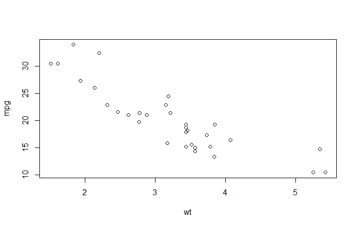
> plot(wt,mpg)
Error in plot(wt, mpg) : object 'wt' not found
> attach(mtcars)
> plot(wt,mpg)
> detach(mtcars)
>#par函数可实现一页多图，颜色。粗细等...

ggplot2中：

> library(ggplot2)
> attach(mtcars)

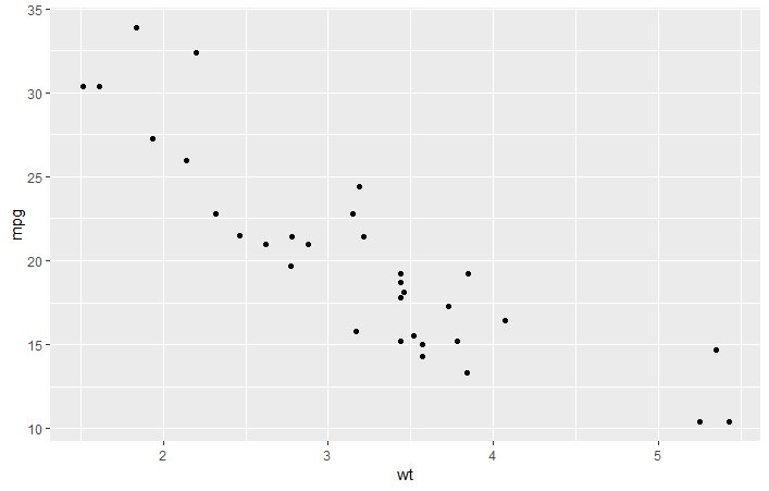
> qplot(wt,mpg)
> detach(mtcars)

等价于：

> qplot(wt,mpg,data=mtcars)

等价于：
> ggplot(mtcars,aes(x=wt,y=mpg))+geom_point()

> ?plot

查看帮助

Usage

plot(x, y, ...)
Arguments

x
the coordinates of points in the plot. Alternatively, a single plotting structure, function or any R object with a plot method can be provided.
y
the y coordinates of points in the plot, optional if x is an appropriate structure.
...
Arguments to be passed to methods, such as graphical parameters (see par). Many methods will accept the following arguments:
type
what type of plot should be drawn. Possible types are
"p" for points,
"l" for lines,
"b" for both,
"c" for the lines part alone of "b",
"o" for both ‘overplotted’,
"h" for ‘histogram’ like (or ‘high-density’) vertical lines,
"s" for stair steps,
"S" for other steps, see ‘Details’ below,
"n" for no plotting.
All other types give a warning or an error; using, e.g., type = "punkte" being equivalent to type = "p" for S compatibility. Note that some methods, e.g. plot.factor, do not accept this.
main
an overall title for the plot: see title.
sub
a sub title for the plot: see title.
xlab
a title for the x axis: see title.
ylab
a title for the y axis: see title.
asp
the y/x aspect ratio, see plot.window.

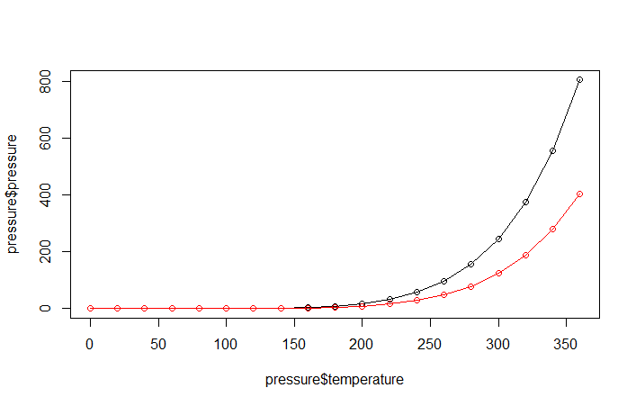
> plot(pressure$temperature,pressure$pressure)

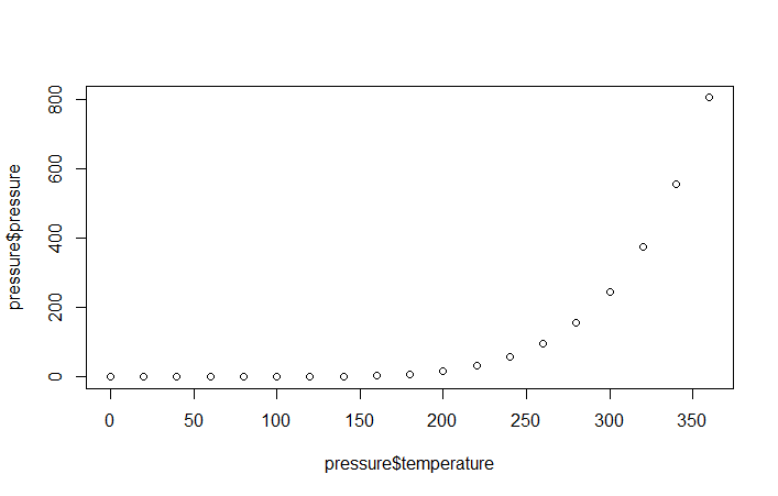
> plot(pressure$temperature,pressure$pressure,type="l")
>

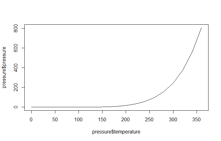
> points(pressure$temperature,pressure$pressure)
>

> lines(pressure$temperature,pressure$pressure/2,col="red")
> points(pressure$temperature,pressure$pressure/2,col="red")
>

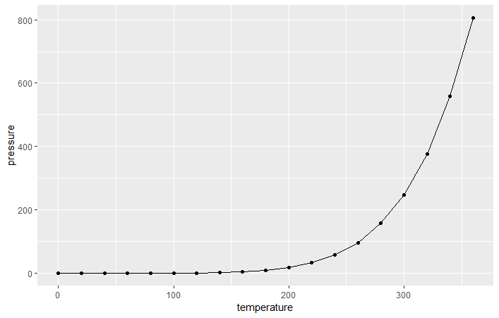
> qplot(pressure$temperature,pressure$pressure,geom="line")
> qplot(temperature,pressure,data=pressure,geom=c("line","point"))
等价于：
> ggplot(pressure,aes(x=temperature,y=pressure))+geom_line()+geom_point()

> data <- mtcars
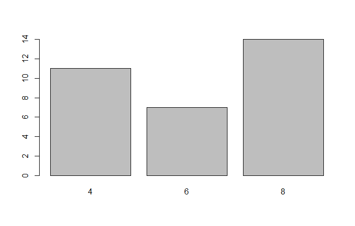
> table(cyl)
cyl
4 6 8
11 7 14

#计算频数

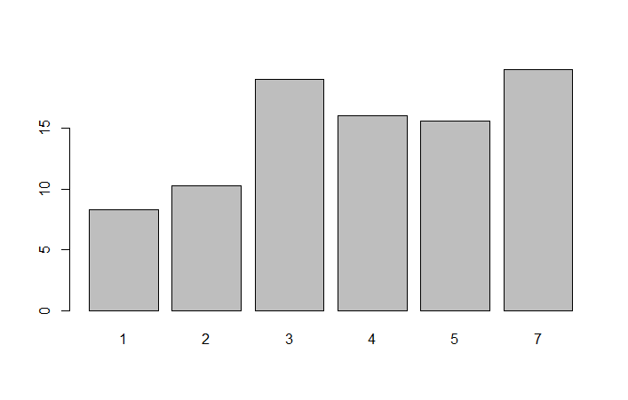
> barplot(BOD$demand,names.arg=BOD$Time)

> barplot(table(cyl))

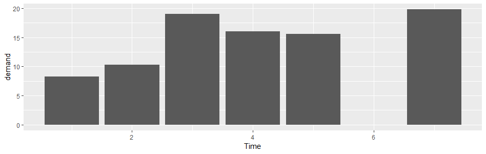
> qplot(BOD$Time,BOD$demand,geom="bar",stat="identity")

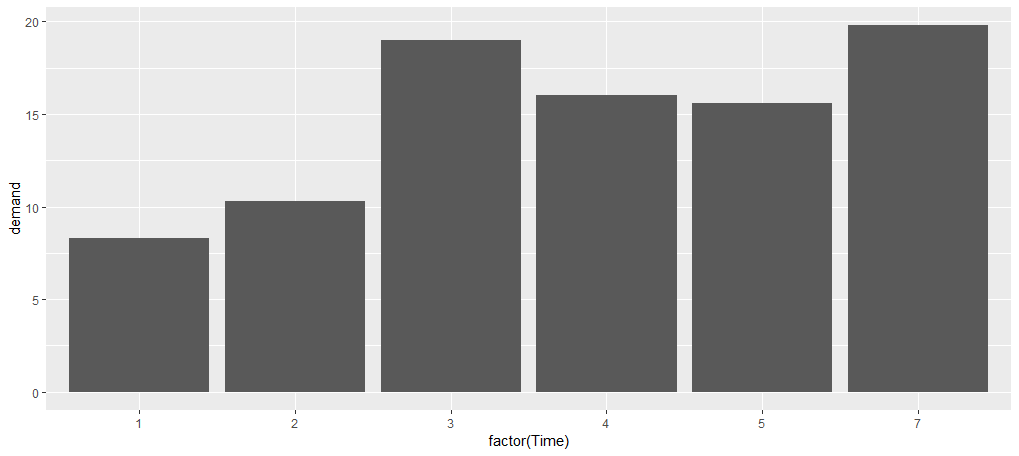
> qplot(factor(BOD$Time),BOD$demand,geom="bar",stat="identity")

绘制不了！

Error: stat_count() must not be used with a y aesthetic.
In addition: Warning message:
`stat` is deprecated

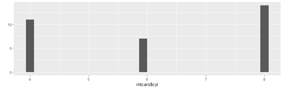
> qplot(mtcars$cyl)

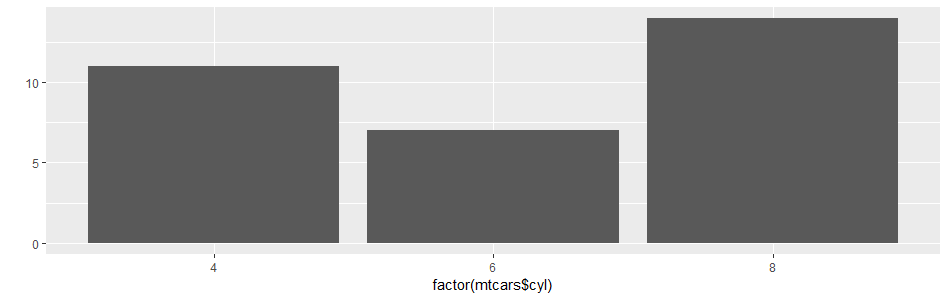
> qplot(factor(mtcars$cyl))

> ggplot(BOD,aes(Time,demand))+geom_bar(stat = 'identity')

> ggplot(BOD,aes(x=factor(Time),y=demand))+geom_bar(stat="identity")
>

https://www.cnblogs.com/lizhilei-123/p/6722116.html

ggplot2之快速作图qplot()----颜色。透明度，形状

频数条形图：

> library(ggplot2)
> ggplot(mtcars,aes(x=factor(cyl)))+geom_bar()

等价：
> qplot(factor(cyl),data=mtcars)

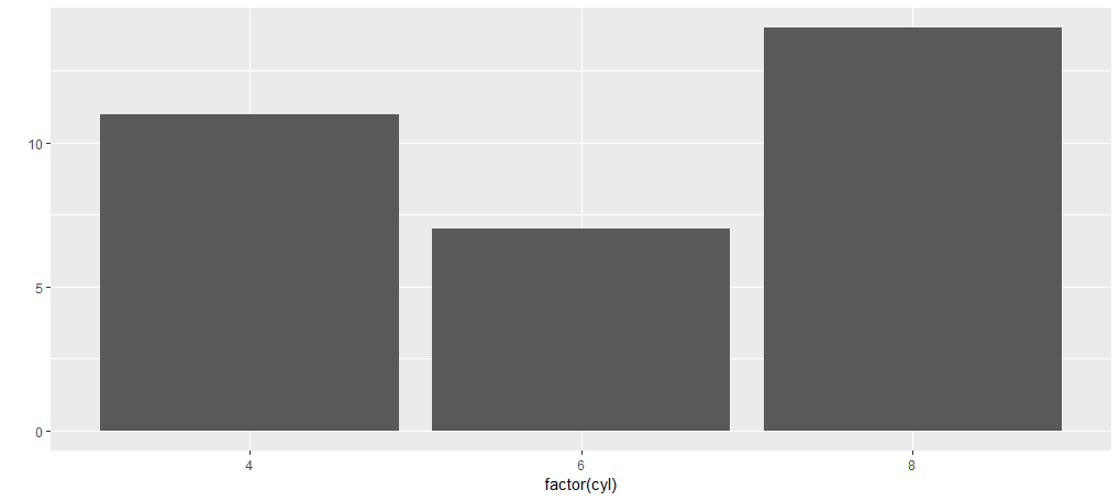
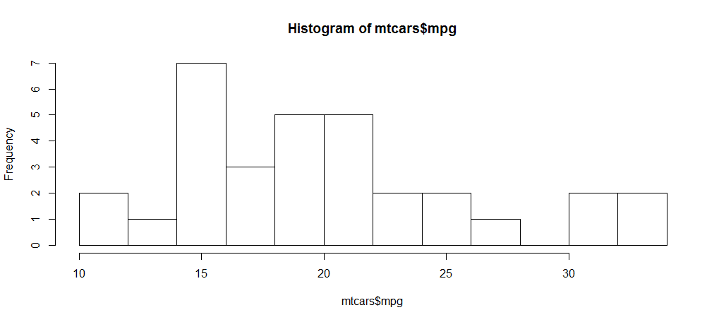
条形图与直方图看起来相似，但是却是不一样的，条形图的x轴是一个确定的数值，而直方图是一个区间。

> hist(mtcars$mpg,breaks=10)

#breaks=10 组距为10

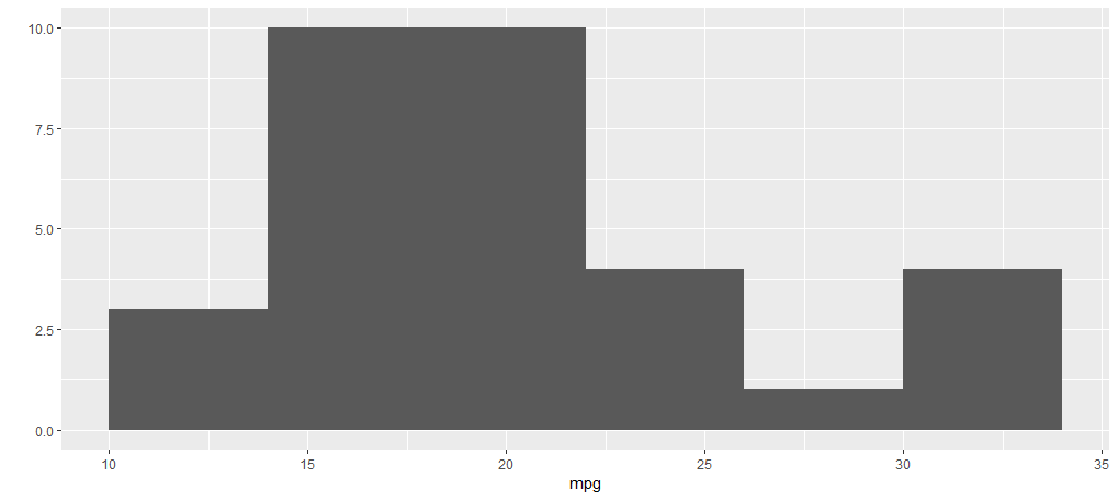
> qplot(mpg,data = mtcars,binwidth=4)

或者

> ggplot(mtcars,aes(x=mpg))+geom_histogram(binwidth = 4)
>binwidth参数是调节横坐标的区间，你可以任意调节你认为合适的区间。

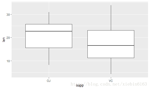
plot(ToothGrowth$supp, ToothGrowth$len)

boxplot(len~supp,data = ToothGrowth)

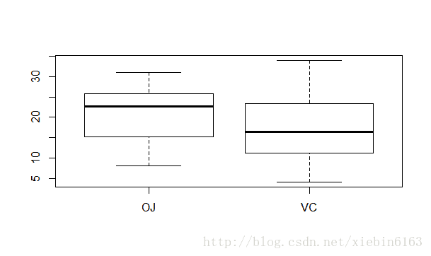
qplot(supp,len,data=ToothGrowth,geom = 'boxplot')

ggplot(ToothGrowth,aes(supp,len))+geom_boxplot()

r code execution error？？？

重装吧。。。。。。。。。。

系统C盘空间容量不够。

R基础--快速探索数据（《R可视化》）

猜你喜欢