BOSS直聘网站数据分析岗位信息爬取

版权声明：本文为博主原创文章，未经博主允许不得转载。 https://blog.csdn.net/qq_27668313/article/details/82924622

          感谢BOSS直聘上比较可靠的招聘信息，让我们有机会对数据分析岗位进行简单的爬取与分析。

语言：Python3

目录

一、信息爬取

二、数据分析

     2.1 数据解析

     2.2 数据分析

         2.2.1 数据清洗

         2.2.2 查看单个特征分布

         2.2.3 分析特征与标签的关系

 三、建模

ps：这里推荐一个学习Python3爬虫非常好的网址，https://cuiqingcai.com/5052.html。内容来自于《Python3网络爬虫开发实战》一书。

首先来参观下页面信息，要爬取的信息有：岗位名称，地区，工作经验，学历，企业信息，薪水。我们会爬取北上广深四个城市的招聘信息。

一、信息爬取

需要导入的库如下，库的安装参考上面给出的链接。

# coding:utf-8
import requests
import csv
import pandas as pd
from bs4 import BeautifulSoup
from requests.exceptions import RequestException

requests相对urllib更加强大，更加友好。虽然与高大上的scrapy相比low了不少，但我们只是从网页上简单爬取一些信息，所以选用requests库。使用BeautifulSoup解析库对爬取的网页信息进行解析。使用pandas.DataFrame将数据保存为csv格式，使用这种方式保存非常方便。

下面我们逐步来完成代码的编写

首先我们需要定义一个函数来获取网站每页的内容。这里使用了一个代理IP。首先，构建一个最简单的GET请求，网站会判断如果客户端发起的是GET请求的话，它返回相应的请求信息。

def get_one_page(url):
	try:
		headers = {
			'User-Agent': 'Mozilla/5.0 (Macintosh; Intel Mac OS X 10_13_3) ' + 
			'AppleWebKit/537.36 (KHTML, like Gecko) Chrome/65.0.3325.162 Safari/537.36'
		}
		html = requests.get(url, headers=headers)
		if html.status_code == 200:
			return html.text
		return None
	except RequestException:
		return None

来看下我们爬取的页面信息源代码长啥样（查看网页源代码的方法这里就不叙述了，网上很多教程），里面的部分黑色字体就是我们要爬取的数据。

获取了一个页面的信息后，就可以对信息进行解析，我们定义一个可以一次解析一个页面的函数，如下。首先定义一个全局变量，用于存储每个公司的招聘信息。（ps:再次说一下，对代码中函数用法不明白的，或者对网页结构不懂的同学，先去文章最上面给出的链接看看）

网页结构可以看成是树结构，上图中<div class='job-primary'>~~</div>可看成一棵子树，包含了一个企业该岗位的全部招聘信息，该子树包含了<div class='info-primary'>~~</div>和<div class='info-company'>~~</div>两个子节点。

下面代码中使用find_all函数获取当前页面中所有<div class='job-primary'>~~</div>子树，即当前页面中所有企业该岗位的招聘信息。通过一个for 循环来遍历companies中的每棵子树，对每棵子树调用parse_one_company()函数进行解析。然后将解析得到的数据存储到result_all列表中。

result_all = [] # 用于存储样本

def parse_one_page(html):
	soup = BeautifulSoup(html, 'lxml')
	companies = soup.find_all('div', 'job-primary', True)
	
	for com in companies:
		res = parse_one_company(com)
		result_all.append(res)

parse_one_company()函数用来对每个<div class='job-primary'>~~</div>子树解析，也就是对每个企业该岗位的招聘信息的解析。在<div class='info-company'>~~</div>节点下解析得到企业所属行业和规模两个信息，即对应网页源代码中的“互联网”和“20-99”。在<div class='info-primary'>~~</div>节点下解析得到岗位名称，薪水，企业地址，工作经验和学历要求信息，即对应网页源代码中的“数据分析师”，“15k-25k”，“广州 番禺区 东环”，“1-3年”，“本科”。最后将这些数据存储到result列表中，并返回。

def parse_one_company(comp):
	result = []
	company_soup = comp.find('div', class_='info-company')
	com_desc = company_soup.find('p').text

	primary_soup = comp.find('div', class_='info-primary')
	job_name = primary_soup.find('div').text
	salary = primary_soup.find('span').text
	requirement = primary_soup.find('p').text

	result.append(com_desc)
	result.append(job_name)
	result.append(salary)
	result.append(requirement)
	return result

上面只是爬取了一个页面一个地区的信息。接下来我们完成要对BOSS直聘上北上广深四个地区的所有数据分析师岗位信息进行爬取。这也是代码的最后一部分。

我们定义了parse_all_page()函数用于爬取四个地区的所有信息。函数中给出了四个地区的url链接，参数num用于指定要爬取的地区，offset参数用于指定要爬取的页面。在最下面的两个for循环中调用parse_all_page()函数。

最后一行生成文件代码中，参数mode='a'可以不用设置，使用mode='w'也可以。encoding='utf_8_sig'一定要设置，否者csv文件会乱码。

def parse_all_page(num, offset):
	
	url1 = 'https://www.zhipin.com/c101280100/h_101280100/?query=数据分析师&page='+str(offset)+'&ka=page-'+str(offset) # 广州
	url2 = 'https://www.zhipin.com/c101280600/h_101280600/?query=数据分析师&page='+str(offset)+'&ka=page-'+str(offset) # 深圳
	url3 = 'https://www.zhipin.com/c101010100/h_101010100/?query=数据分析师&page='+str(offset)+'&ka=page-'+str(offset) # 北京
	url4 = 'https://www.zhipin.com/c101020100/h_101020100/?query=数据分析师&page='+str(offset)+'&ka=page-'+str(offset) # 上海
	urldict = {'1':url1, '2':url2, '3':url3, '4':url4}

	html = get_one_page(urldict[str(num)])
	parse_one_page(html)
	


if __name__ == '__main__':
	for j in range(1, 5):
		for i in range(1,11):
			parse_all_page(j, i)
	file = pd.DataFrame(result_all, columns=['公司信息', '岗位', '薪水', '其他'])
	# encoding='utf_8_sig解决保存到CSV文件后显示乱码问题
	file.to_csv('Bosszhiping_four_city.csv', mode='a', index=True, encoding='utf_8_sig')

至此，代码已完成！Python爬虫有很多种方法，只要掌握一种即可，如果只是对网页进行爬取，requests库就可以满足了，如果是对整个网站进行爬取，那就得用scrapy了。

二、数据分析

2.1 数据解析

import numpy as np
import pandas as pd
import matplotlib.pyplot as plt
import re

# 导入数据，第一列的序号不导入
data_df = pd.read_csv('Bosszhiping_four_city.csv', usecols=[1,2,3,4])

# 查看数据前5行信息，简单了解下数据
data_df.head()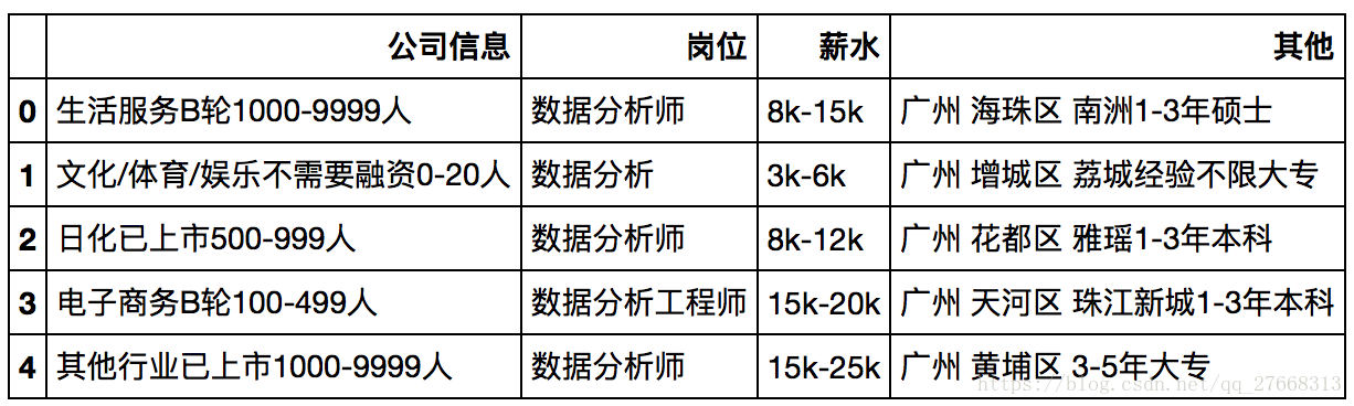

表中“公司信息”和“其他”特征存在多种信息，因此需要对其进行解析。

首先对“其他”特征进行解析，目的是得到“城市”，“城区”，“工作经验”，“学历”四个特征

others = list(data_df['其他'])
others[0:5]

# 工作经验和学历没有空格隔开，我们暂时将两者放到edu列表中
city, area, edu= [], [], []
leng = len(others)
for s in others:
    temp = s.split(' ')
    city.append(temp[0])
    area.append(temp[1])
    edu.append(temp[2])
print(city[0:5])
print(area[0:5])
print(edu[0:5])
print(len(city), len(area), len(edu))

# 对edu列表进一步解析，得到“工作经验”和“学历”特征
for i in range(leng):
    edu[i] = edu[i].replace('应届生','0-Graduate ')
    edu[i] = edu[i].replace('经验不限', '0-Unlimited ')
    edu[i] = edu[i].replace('年', ' ') 
experience = [] # 经验特征
education = [] # 学历特征
for s in edu:
    temp = s.split(' ')
    experience.append(temp[0])
    education.append(temp[1][-2:])
print(experience[0:10])
print(education[0:10])

for i in range(leng):
    temp = re.findall(r'\d\-?\d?\w*', experience[i]) # 使用正则表达式
    if len(temp) != 0:
        experience[i] = temp[0]
    else:
        experience[i] = None
print(experience[0:10])

然后对“公司信息”特征进行解析，目的是得到“所属行业”，“是否上市”，“企业规模”特征

company = list(data_df['公司信息'])
print(company[0:5])

# 获取企业规模特征
CompSize = [None] * leng #企业规模
for i in range(leng):
    temp = re.findall(r'\d+\-?\d+', company[i])
    if temp is not None:
        CompSize[i] = temp[0]
print(CompSize[0:5])

# 获取企业是否上市特征，上市为1，非上市为0
CompType = [0] * leng # 企业类型,是否上市
for i in range(leng):
    if '已上市' in company[i]:
        CompType[i] = 1
print(CompType[0:10])

# 获取企业所属行业特征
# 由于MAC 的matplotlib中文显示问题，将中文换成英文
IndustryCate = [None] * leng # 企业所属行业
for i in range(leng):
    # 不能使用 if '互联网' or ‘网络’ in company[i]:
    # 因为 '互联网' or ‘网络’ 这构成一个判断语句，两边都非空，因此输出True, if条件中永远成立。
    if '电子商务' in company[i]:
        IndustryCate[i] = 'E-Commerence'
    elif '互联网' in company[i]:
        IndustryCate[i] = 'Internet' 
    elif '网络' in company[i]:
        IndustryCate[i] = 'Internet'
    elif '计算机' in company[i]:
        IndustryCate[i] = 'Computer soft'
    elif '数据服务' in company[i]:
        IndustryCate[i] = 'Data service'
    elif '医疗' in company[i]:
        IndustryCate[i] = 'Medical care'
    elif '健康' in company[i]:
        IndustryCate[i] = 'Medical care'
    elif '游戏' in company[i]:
        IndustryCate[i] = 'Game'
    elif '教育' in company[i]:
        IndustryCate[i] = 'Education'
    elif '生活' in company[i]:
        IndustryCate[i] = 'Life service'
    elif '旅游' in company[i]:
        IndustryCate[i] = 'Life service'
    elif '物流' in company[i]:
        IndustryCate[i] = 'Logistics'
    elif '广告' in company[i]:
        IndustryCate[i] = 'Advertisement'
    elif '零售' in company[i]:
        IndustryCate[i] = 'Retail'
    elif '咨询' in company[i]:
        IndustryCate[i] = 'Consulting'
    elif '进出口' in company[i]:
        IndustryCate[i] = 'Foreign trade'
    else:
        IndustryCate[i] = 'Others'

print(IndustryCate[0:10])

salary = list(data_df['薪水'])
salary_int = [] 
salary_str = [0] * leng
for s in salary:
    temp = re.findall(r'\d+', s)
    temp1 = int(temp[0])
    temp2 = int(temp[1])
    #print(temp1, temp2)
    avg = (temp2 + temp1)/2
    #print(avg)
    salary_int.append(avg)
    
for i in range(len(salary)):
    if salary_int[i] <= 6:
        salary_str[i] = '0-6k'
    elif salary_int[i] > 6 and salary_int[i] <= 10:
        salary_str[i] = '6-10k'
    elif salary_int[i] >10 and salary_int[i] <= 15:
        salary_str[i] = '10-15k'
    elif salary_int[i] > 15 and salary_int[i] <=20:
        salary_str[i] = '15-20k'
    elif salary_int[i] > 20 and salary_int[i] <=30:
        salary_str[i] = '20-30k'
    elif salary_int[i] >30:
        salary_str[i] = '30+k'

print(salary_int[0:5])
print(salary_str[0:5])  

特征解析完成后，将新得到的特征和原来的“岗位”，“薪水”特征一起组成一个新的数据

#education_ = list(data_df['学历'])
education = map(lambda s:[s, 'Doctor'][s=='博士'], education)
education = map(lambda s:[s, 'Master'][s=='硕士'], education)
education = map(lambda s:[s, 'Undergraduate'][s=='本科'], education)
education = map(lambda s:[s, 'Specialty'][s=='大专'], education)
education = map(lambda s:[s, 'Second special'][s=='中技'], education)
education = map(lambda s:[s, 'High school'][s=='高中'], education)
education = map(lambda s:[s, 'Unlimited'][s=='不限'], education)
education = list(education)
job = list(data_df['岗位'])
dicts = {'岗位':job, '城市':city, '城区':area, '经验/年':experience, '企业规模/人':CompSize, \
         '学历':education, '是否上市':CompType, '所属行业':IndustryCate, '薪水str':salary_str, '薪水int/k':salary_int}
newdata = pd.DataFrame(dicts)
newdata.head()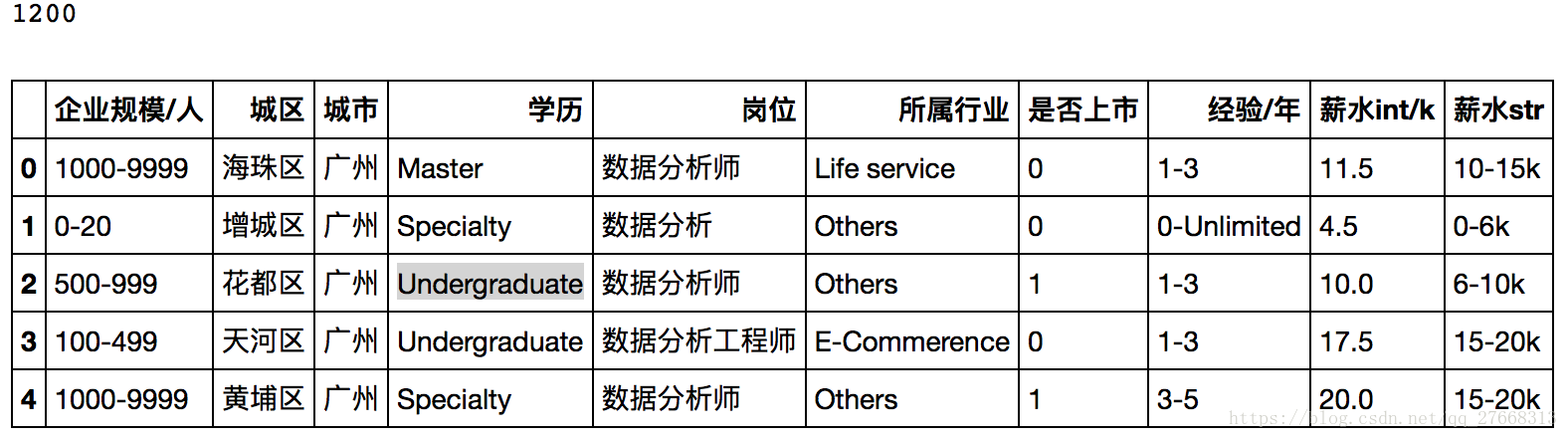

# 生成文件
newdata.to_csv('newDataEng.csv', encoding='utf_8_sig')

2.2 数据分析

import numpy as np
import pandas as pd
import re
import matplotlib.pyplot as plt
import matplotlib as mpl
from pyecharts import Map

2.2.1 数据清洗

# 加载数据
data = pd.read_csv('newDataEng.csv')

data.head()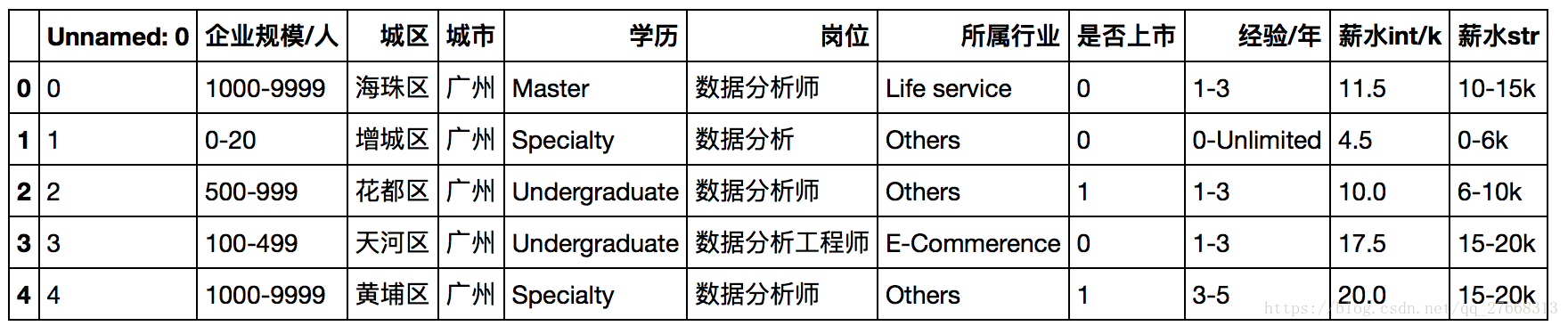

leng = len(data)
print(leng)

1200

# 删除实习生岗位
job = data['岗位']
j = 0
for i in range(leng):
    if '实习生' in job[i]:
        j += 1 
        data.drop(axis=0, index=i, inplace=True)
leng = len(data)
print(j, leng)

29， 1171

data.info()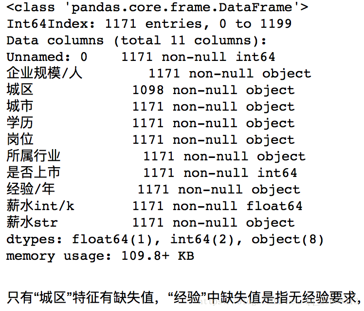

2.2.2 查看单个特征分布

# 查看学历分类及分布
data['学历'].value_counts()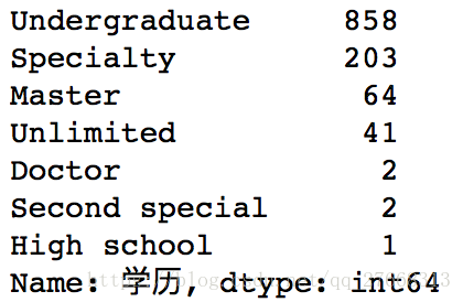

labels = list(data['学历'].value_counts().index)
fracs = list(data['学历'].value_counts().values)
explode = [0, 0.1, 0.2, 0.3, 0.5, 1.5, 2.8]
plt.pie(x=fracs, labels=labels, explode=explode, autopct='%.3f')
plt.show()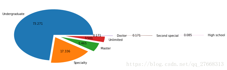

主要以本科学历为主，说明该岗位工作难度不大

# 查看经验分布
data['经验/年'].value_counts()

由于是社招招聘信息，所以有工作经验要求，1-3，3-5年为主

labels = list(data['经验/年'].value_counts().index)
fracs = list(data['经验/年'].value_counts().values)
explode = [0, 0.1, 0.2, 0.3, 0.5, 1, 1.5]
plt.pie(x=fracs, labels=labels, explode=explode, autopct='%.3f')
plt.show()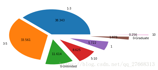

# 查看企业规模分布
data['企业规模/人'].value_counts().plot(kind='bar')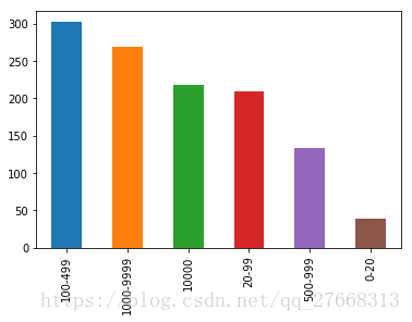

岗位大都来自于中大型企业，小企业需求少

# 查看企业类型分布
data['是否上市'].value_counts().plot(kind='bar')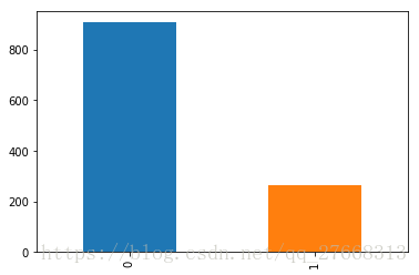

# 查看企业所属行业分布
data['所属行业'].value_counts().plot(kind='barh')

以互联网企业居多，远超其他行业类企业。说明互联网企业更注重数据价值，或者是互联网企业流量更多

# 查看薪水分布
data['薪水str'].value_counts()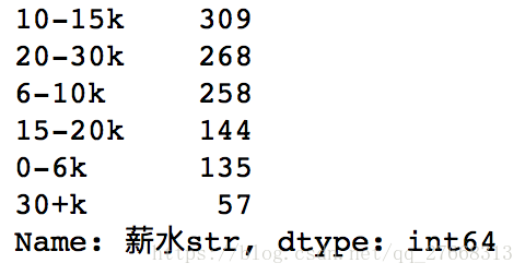

labels = list(data['薪水str'].value_counts().index)
fracs = list(data['薪水str'].value_counts().values)
plt.pie(x=fracs, labels=labels, autopct='%.3f')
plt.show()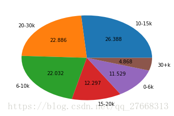

# 企业所属行业词云图
import wordcloud
word_list = list(data['所属行业'])
word = ''
for s in word_list:
    word = word + s + ' '
print(word[0:100])
mywc = wordcloud.WordCloud(width=600, height=400, min_font_size=20).generate(word)
plt.imshow(mywc, interpolation='bilinear')
plt.axis('off')
plt.imsave('HangyeWordC.png', mywc)

# 查看广州市各区岗位数量
area_job = data['城区'].groupby(data['城市']).value_counts()
area_city = list(area_job['广州'].index)
area_num = list(area_job['广州'].values)
map = Map('广州市各区岗位分布图', width=1200, height=600)
map.add('', area_city, area_num, visual_range=[0, 150], visual_text_color='#000', is_visualmap=True,
        is_label_show=True, maptype='广州')
#map.render('./job_city_area.html')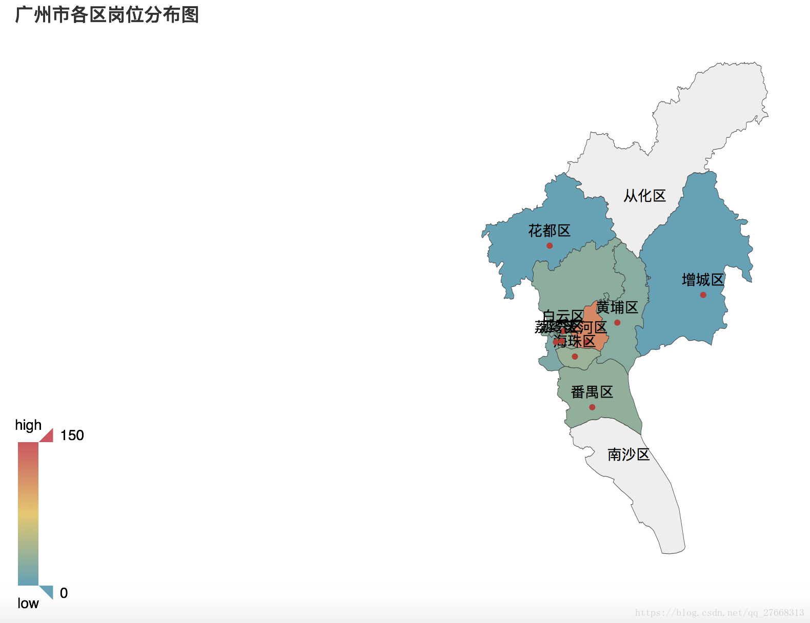

天河区企业数量最多

2.2.3 分析特征与标签的关系

# 定义特征-薪水柱状图
def plotbar(data_list, data_sala, m, n, stack=False):
    # data_list 特征变量种类， data_sala 薪水按特征分组后的数据
    # (m, n) 设置图片大小，stack设置是否使用堆叠柱状图
    xlabel_list = ['0-6k', '6-10k', '10-15k', '15-20k', '20-30k', '30+k']
    n = len(xlabel_list)
    lengSize = len(data_list)
    total_width = 0.8
    width = total_width / n
    x = np.arange(n)
    x = x - (total_width - width) / 2

    plt.figure(figsize=(m, n))
    #num_list = [0] * n
    for j in range(lengSize):
        num_list = [0] * n
        init_num_list = list(data_sala[data_list[j]].values)
        index_list = list(data_sala[data_list[j]].index)
        # 用0补充缺失值
        for i in range(len(index_list)):
            if index_list[i] in xlabel_list:
                index = xlabel_list.index(index_list[i])
                num_list[index] = init_num_list[i]
        if stack:
            plt.bar(x, num_list, width=width, label=data_list[j])
        else:
            plt.bar(x+j*width, num_list, width=width, label=data_list[j])
        # 设置横坐标刻度标签
        plt.xticks(x, xlabel_list)
        plt.legend()

# 是否上市与薪水关系
comType_list = list(data['是否上市'].value_counts().index)
comType_sala = data['薪水str'].groupby(data['是否上市']).value_counts(sort=False) 
plotbar(comType_list, comType_sala, 10, 8, False)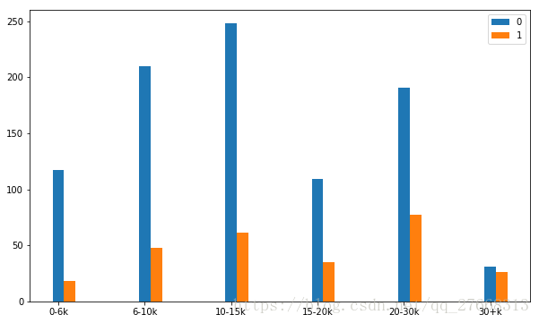

# 企业规模与薪水的关系
comSize_list = list(data['企业规模/人'].value_counts().index)
comSize_sala = data['薪水str'].groupby(data['企业规模/人']).value_counts(sort=False)
plotbar(comSize_list, comSize_sala, 15, 8)

# 定义折线-柱状图函数
def plotlinebar(dataType_list, data_sala, data_num):
    # dataType_list 横坐标轴， data_sala 特征下的平均薪水， data_num 数据在特征下分组的数量
    dataType_sala = []
    for i in range(len(dataType_list)):
        numa = list(data_sala[dataType_list[i]].index)
        numb = list(data_sala[dataType_list[i]].values)
        result = sum(np.multiply(np.array(numa), np.array(numb)))/sum(numb)
        dataType_sala.append(result)
    
    ax1 = plt.figure(figsize=(10,8)).add_subplot(111)
    plt.xticks(range(len(dataType_list)), dataType_list) # 防止折线图点连接顺序混乱，自定义横坐标刻度
    ax1.plot(dataType_sala, 'or-')
    ax1.set_ylabel('Mean salary k/month')

    ax2 = ax1.twinx()
    ax2.bar(range(len(dataType_list)),data_num, alpha=0.5) #上面已经自定义了横坐标轴，这里与其保持一致
    ax2.set_ylabel('numbers')

    plt.show()

# 学历与薪水关系
eduType_list = list(data['学历'].value_counts().index)
edu_sala = data['薪水int/k'].groupby(data['学历']).value_counts(sort=False)
edu_num = list(data['学历'].value_counts())
plotlinebar(eduType_list, edu_sala, edu_num)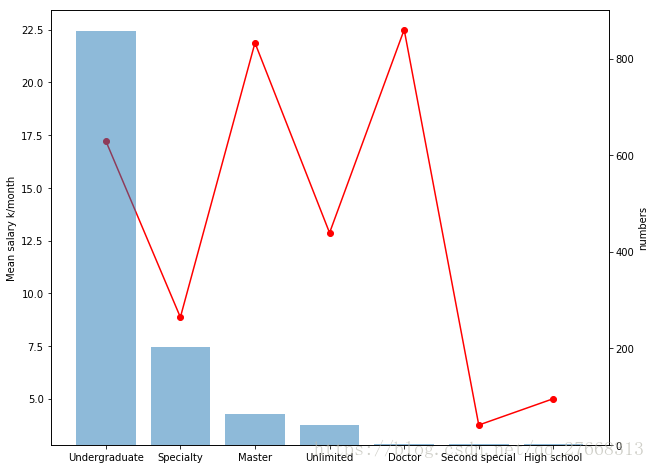

# 经验与薪水的关系
expType_list = list(data['经验/年'].value_counts().index)
exp_sala = data['薪水int/k'].groupby(data['经验/年']).value_counts(sort=False)
exp_num = list(data['经验/年'].value_counts())
plotlinebar(expType_list, exp_sala, exp_num)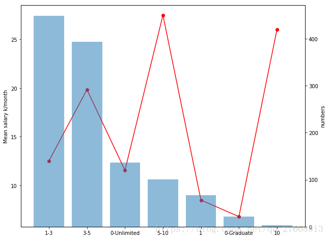

#coding:utf-8
import seaborn as sns
import matplotlib as mpl
#mpl.rcParams['font.sans-serif'] = ['simhei']
#mpl.rcParams['axes.unicode_minus'] = False 
# 广州不同地区薪酬比较
gz_data = data[data['城市']=='广州']
sns.boxplot(x=gz_data['城区'], y=gz_data['薪水int/k'])
# matplotlib中文显示乱码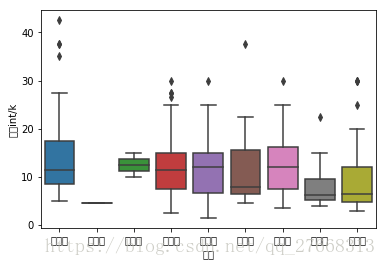

# 定义雷达图函数
def plotlinebar(dataType_list, data_sala, data_num):
    # dataType_list 横坐标轴， data_sala 特征下的平均薪水， data_num 数据在特征下分组的数量
    dataType_sala = []
    for i in range(len(dataType_list)):
        numa = list(data_sala[dataType_list[i]].index)
        numb = list(data_sala[dataType_list[i]].values)
        result = sum(np.multiply(np.array(numa), np.array(numb)))/sum(numb)
        dataType_sala.append(result)
    dataType_sala = np.array(dataType_sala)
    
    angles = np.linspace(0, 2*np.pi, len(dataType_list), endpoint=False)
    data = np.concatenate((dataType_sala, [dataType_sala[0]]))
    angles = np.concatenate((angles, [angles[0]]))
                            
    ax = plt.figure(figsize=(10, 10)).add_subplot(111, polar=True)
    ax.plot(angles, data, 'bo-', linewidth=2)
    ax.fill(angles, data, facecolor='r', alpha=0.3)
    ax.set_thetagrids(angles*180/np.pi, dataType_list)    
    plt.show()

# 所属行业与薪水关系
indcateType_list = list(data['所属行业'].value_counts().index)
indcate_sala = data['薪水int/k'].groupby(data['所属行业']).value_counts()
indcate_num = list(data['所属行业'].value_counts())
plotlinebar(indcateType_list, indcate_sala, indcate_num)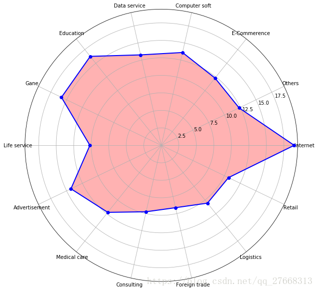

三、 建模

from sklearn.model_selection import train_test_split, cross_val_score, learning_curve
from sklearn.linear_model import LogisticRegression, LinearRegression
from sklearn.svm import SVC
from sklearn.neighbors import KNeighborsClassifier, KNeighborsRegressor
from sklearn.metrics import accuracy_score, mean_squared_error
import seaborn as sns
import warnings

warnings.filterwarnings('ignore')

划分特征和标签，薪水str是分类问题

label_str = data['薪水str']
train_data = data.drop(columns=['岗位', '薪水int/k', '薪水str'])
# one-hot 编码
train_data = pd.get_dummies(train_data)
# 学习曲线图
train_sizes, tr_loss, te_loss = learning_curve(LogisticRegression(), train_data, label_str,\
                                              cv=10, scoring='accuracy')
tr_loss_m = np.mean(tr_loss, axis=1)
te_loss_m = np.mean(te_loss, axis=1)

plt.figure()
plt.plot(train_sizes, tr_loss_m, 'o-', color='r', label='train acc')
plt.plot(train_sizes, te_loss_m, 'o-', color='b', label='test acc')
plt.xlabel('train sizes')
plt.ylabel('accuracy')
plt.legend(loc='best')


# 划分分类问题的训练集和测试集
train_xs, test_xs, train_ys, test_ys = train_test_split(train_data, label_str, test_size=0.25)

model_lr = LogisticRegression()
scores = cross_val_score(model_lr, train_xs, train_ys, scoring='accuracy', cv=5)
model_lr.fit(train_xs, train_ys)
pred_lr = model_lr.predict(test_xs)
print(accuracy_score(test_ys, pred_lr))

0.4402730375426621

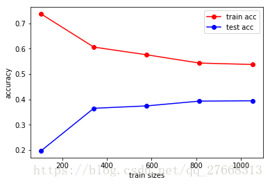
一点点说明

模型预测结果差，是因为样本不具备代表性，存在太多噪音，标签的设定也有待商榷。

本文只从BOSS直聘网站上爬取了信息，这直接导致样本不能代表全网站的招聘信息。BOSS网站上只显示了30页数据，因此爬取的样本甚至都不能代表BOSS直聘上发布的招聘信息。这两点导致样本不具备代表性。

标签的没有统一的规定，各个企业给出的薪水范围没有具体的标准，导致难以设计薪水等级。