IMDB数据集是Keras内部集成的,初次导入需要下载一下,之后就可以直接用了。
IMDB数据集包含来自互联网的50000条严重两极分化的评论,该数据被分为用于训练的25000条评论和用于测试的25000条评论,训练集和测试集都包含50%的正面评价和50%的负面评价。该数据集已经经过预处理:评论(单词序列)已经被转换为整数序列,其中每个整数代表字典中的某个单词。
加载数据集
from keras.datasets import imdb

(train_data, train_labels), (test_data, test_labels) = imdb.load_data(num_words=10000)
参数num_words = 10000的意思是仅保留训练数据的前10000个最常见出现的单词,低频单词将被舍弃。这样得到的向量数据不会太大,便于处理。
train_data[0]
[1,
14,
22,
16,
43,
530,
973,
1622,
1385,
65,
458,…
train_labels[0]
0表示负面,1表示正面。
下面的代码可以将某条评论迅速解码为英文单词:
# word_index is a dictionary mapping words to an integer index
word_index = imdb.get_word_index()
# We reverse it, mapping integer indices to words
reverse_word_index = dict([(value, key) for (key, value) in word_index.items()])
# We decode the review; note that our indices were offset by 3
# because 0, 1 and 2 are reserved indices for "padding", "start of sequence", and "unknown".
decoded_review = ' '.join([reverse_word_index.get(i - 3, '?') for i in train_data[0]])
我们这里,key是单词,value是数字,转换索引之后,就让数字变成键了。我们使用join方法,使用空格来分隔每个单词。
展示结果如下:
"? this film was just brilliant casting location scenery story direction everyone’s really suited the part they played and you could just imagine being there robert ? is an amazing actor and now the same being director ? father came from the same scottish island as myself so i loved the fact there was a real connection with this film the witty remarks throughout the film were great it was just brilliant so much that i bought the film as soon as it was released for ? and would recommend it to everyone to watch and the fly fishing was amazing really cried at the end it was so sad and you know what they say if you cry at a film it must have been good and this definitely was also ? to the two little boy’s that played the ? of norman and paul they were just brilliant children are often left out of the ? list i think because the stars that play them all grown up are such a big profile for the whole film but these children are amazing and should be praised for what they have done don’t you think the whole story was so lovely because it was true and was someone’s life after all that was shared with us all"
准备数据
我们不能将整数序列直接输入神经网络,需要先将列表转换为张量。转换方式有以下两种:
-
填充列表
-
对列表进行one-hot编码 :比如序列[3, 5]将会被转换为10000维向量,只有索引为3和5的元素是1,其余元素是0,然后网络第一层可以用Dense层,它能够处理浮点数向量数据。
这里,我们采用one-hot编码的方式进行。
import numpy as np

def vectorize_sequences(sequences, dimension=10000):

    results = np.zeros((len(sequences), dimension))
    for i, sequence in enumerate(sequences):
        results[i, sequence] = 1.  # 索引results矩阵中的位置,赋值为1,全部都是从第0行0列开始的
    return results

# Our vectorized training data
x_train = vectorize_sequences(train_data)
# Our vectorized test data
x_test = vectorize_sequences(test_data)
x_train[0]
样本变成了如下样子:
array([ 0., 1., 1., …, 0., 0., 0.])
还需要将标签向量化
y_train = np.asarray(train_labels).astype('float32')
y_test = np.asarray(test_labels).astype('float32')
下面可以把数据输入神经网络了。
构建网络
from keras import models
from keras import layers

model = models.Sequential()
model.add(layers.Dense(16, activation='relu', input_shape=(10000,)))
model.add(layers.Dense(16, activation='relu'))
model.add(layers.Dense(1, activation='sigmoid'))
最后需要选择损失函数和优化器,由于面对的是一个二分类问题,网络输出是一个概率值,那么最好使用binary_crossentropy(二元交叉熵)。对于输出概率值的模型,交叉熵(crossentropy)往往是最好的选择。
model.compile(optimizer='rmsprop',
              loss='binary_crossentropy',
              metrics=['accuracy'])
有时你可能希望配置自定义优化器的参数,或传入自定义的损失函数或指标函数。前者可以通过向optimizer参数传入一个优化器类实例来实现,后者可以通过向losshemetric参数传入函数对象来实现。
from keras import optimizers

model.compile(optimizer=optimizers.RMSprop(lr=0.001),
              loss='binary_crossentropy',
              metrics=['accuracy'])
from keras import losses
from keras import metrics

model.compile(optimizer=optimizers.RMSprop(lr=0.001),
              loss=losses.binary_crossentropy,
              metrics=[metrics.binary_accuracy])
验证
在训练过程中对模型进行监控,将原始训练集留出10000个样本作为验证集。
x_val = x_train[:10000]
partial_x_train = x_train[10000:]

y_val = y_train[:10000]
partial_y_train = y_train[10000:]
下面使用512个样本组成的小批量,将模型训练20次。与此同时,还要监控留出的10000个样本上的损失函数和精度,可以通过将验证数据传入validation_data参数来完成。
history = model.fit(partial_x_train,
                    partial_y_train,
                    epochs=20,
                    batch_size=512,
                    validation_data=(x_val, y_val))
当我们调用model.fit()的时候,返回一个History对象。这个对象有一个成员history,它是一个字典,包含训练过程中的所有数据。
history_dict = history.history
history_dict.keys()
输出:dict_keys([‘val_acc’, ‘acc’, ‘val_loss’, ‘loss’])
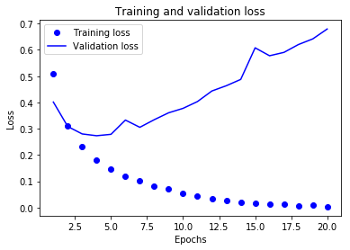
我们下面在matplotlib中用同一张图绘制训练损失和验证损失,以及训练精度和验证精度。
import matplotlib.pyplot as plt

acc = history.history['acc']
val_acc = history.history['val_acc']
loss = history.history['loss']
val_loss = history.history['val_loss']

epochs = range(1, len(acc) + 1)

# "bo" is for "blue dot"
plt.plot(epochs, loss, 'bo', label='Training loss')  # bo表示蓝色圆点
# b is for "solid blue line"
plt.plot(epochs, val_loss, 'b', label='Validation loss')  # b表示蓝色实线
plt.title('Training and validation loss')
plt.xlabel('Epochs')
plt.ylabel('Loss')
plt.legend()  #如果不加这一句就不会显示图例

plt.show()
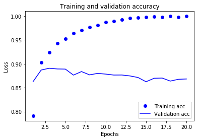
plt.clf()   # clear figure
acc_values = history_dict['acc']
val_acc_values = history_dict['val_acc']

plt.plot(epochs, acc, 'bo', label='Training acc')
plt.plot(epochs, val_acc, 'b', label='Validation acc')
plt.title('Training and validation accuracy')
plt.xlabel('Epochs')
plt.ylabel('Loss')
plt.legend()

plt.show()
最终训练和用于预测
重新写一遍整个训练模型代码
model = models.Sequential()
model.add(layers.Dense(16, activation='relu', input_shape=(10000,)))
model.add(layers.Dense(16, activation='relu'))
model.add(layers.Dense(1, activation='sigmoid'))

model.compile(optimizer='rmsprop',
              loss='binary_crossentropy',
              metrics=['accuracy'])

model.fit(x_train, y_train, epochs=4, batch_size=512)
results = model.evaluate(x_test, y_test)
最终results输出的结果是:
[0.29184698499679568, 0.88495999999999997]
我们得到了88%的精度。
如果我们想要用于预测,可以使用predict方法:
model.predict(x_test)
array([[ 0.91966152],
[ 0.86563045],
[ 0.99936908],
…,
[ 0.45731062],
[ 0.0038014 ],
[ 0.79525089]], dtype=float32)
更多精彩内容,欢迎关注我的微信公众号:数据瞎分析