深度学习 从零开始 —— 神经网络（四），二分类问题，IMDB数据集使用

IMDB数据集

互联网电影数据，包含50000条严重两极分化的评论。正面和负面评论各占50%。
而该数据集也同样被内置于Keras库中了。

其中的评论数据已经经过了预处理，评论（单词）被转化为了整数序列，每个整数都对应词典里面的一个单词。

加载数据集

from keras.datasets import imdb

(train_data,train_labels),(test_data,test_labels) = imdb.load_data(num_words=10000)
#第一条评论的单词索引列表
print(train_data[0])
#1表示正面品论，0表示负面评论
print(train_labels[0])
#取所有测试单词所有的最大的索引值
print(max([max(sequence) for sequence in train_data]))

num_words=10000是取最常出现的10000个单词，舍弃低频词语。减小向量数据量。
train_data和test_data都是评论的列表（单词索引组成）。
train_labels和test_labels都是0和1组成的列表。
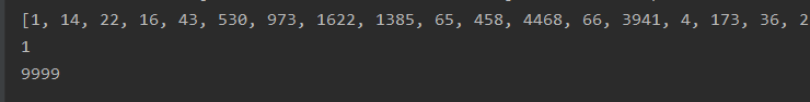可以看到最大9999就是说索引不超过10000

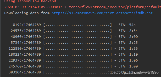
第一次加载时会下载数据集

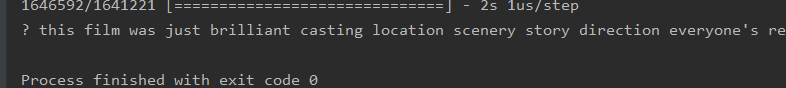
解码为英语

#某条评论解码为英文
word_index = imdb.get_word_index()
reverse_word_index = dict(
    [(value,key) for (key,value) in word_index.items()]
)
decoded_review = ' '.join(
    [reverse_word_index.get(i-3,'?') for i in train_data[0]]
)
print(decoded_review)

imdb.get_word_index()这个是单词映射整数的字典，将其键值颠倒，变为根据索引查单词。
其中i-3是因为0,1,2是为填充，序列开始，未知词保留的索引

处理数据

import numpy as np

#转换为10000维的向量，索引的位置是1，其他位置是0
def vectorize_sequences(sequences,dimension=10000):
    results = np.zeros((len(sequences),dimension))
    for i, sequence in enumerate(sequences):
        results[i,sequence] = 1.
    return results
#数据向量化
x_train = vectorize_sequences(train_data)
x_test = vectorize_sequences(test_data)
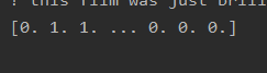
print(x_train[0])
#标签向量化
y_train = np.asarray(train_labels).astype('float32')
y_test = np.asarray(test_labels).astype('float32')

将每一条评论的索引值转化到10000维向量上。有该索引值的设为1，其余位置设为0.
例如一条评论为[1,3,5]，则变为[0,1,0,1,0,1,0,0,0,0…,0]。

建立网络

from keras import models
from keras import layers

#模型定义
model = models.Sequential()
model.add(layers.Dense(16,activation='relu',input_shape=(10000,)))
model.add(layers.Dense(16,activation='relu'))
model.add(layers.Dense(1,activation='sigmoid'))
#定义优化器，损失函数，指标
model.compile(optimizer='rmsprop',
              loss='binary_crossentropy',
              metrics=['accuracy'])

模型为三层。

• 一二层都是16个隐藏单元，输入10000维的向量。做的操作除了张量的操作外，relu是激活函数之一，将线性的变换集合变成非线性。
• 第三层输出1维，sigmod是将输出归一化，变成[0,1]的概率。

二分类问题，输出是一个概率值（正面评价的概率）。
因此选用交叉熵（crossentropy）来计算损失。
而优化器使用rmsprop。这是前任总结的最优于此示例的，至于为什么选这两个，后面章节在做学习。

验证集

为了在训练过程中监控模型对于未见过的数据上的精度，从数据中去出10000个样本用来做验证集。

#取10000用于验证集
x_val = x_train[:10000] #验证集
partial_x_train = x_train[10000:]

y_val = y_train[:10000] #验证集
partial_y_trail = y_train[10000:]

训练模型

#训练模型
history = model.fit(partial_x_train,
                    partial_y_trail,
                    epochs=20,
                    batch_size=512,
                    validation_data=(x_val,y_val))
                    
history_dict = history.history
print(history_dict.keys())

我们输入训练数据集partial_x_train，训练标签集partial_y_trail。
全部数据训练次数*20。
一次取512的个数据。
history 中包含了训练过程中的所有数据。
validation_data是前一步取出来的验证集。

history包含训练过程中的所有数据。打印history_dict所包含的指标。

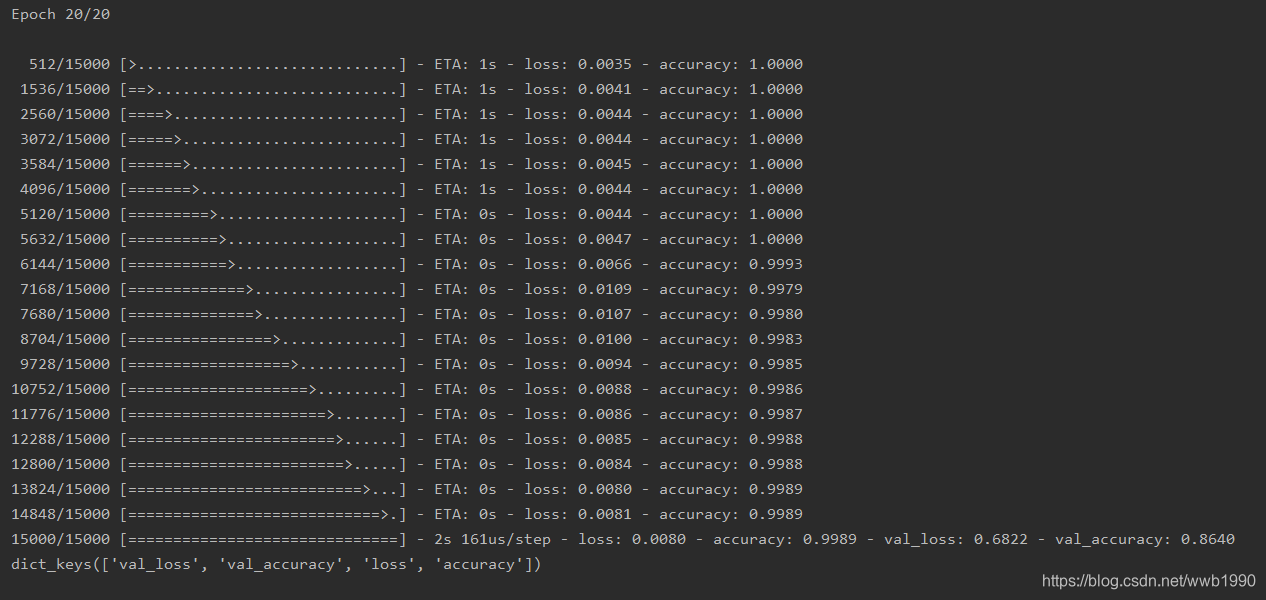
可以看到其中包括验证精度，训练精度，验证损失，训练损失。

我们来用matplot绘制出这几个指标的走势：

损失变化图：

loss_values = history_dict['loss']
val_loss_values = history_dict['val_loss']

epochs = range(1,len(loss_values)+1)

plt.plot(epochs,loss_values,'bo',label='Training loss') #bo是蓝色圆点
plt.plot(epochs,val_loss_values,'b',label='Validation loss') #b是蓝色实线
plt.title('Training and validation loss')
plt.xlabel('Epochs')
plt.ylabel('Loss')
plt.legend()
plt.show()

精度变化图：

plt.clf() #清空图表

acc_values = history_dict['acc']
val_acc_values  = history_dict['val_acc']

plt.plot(epochs,acc_values,'bo',label='Training acc') #bo是蓝色圆点
plt.plot(epochs,val_acc_values,'b',label='Validation acc') #b是蓝色实线
plt.title('Training and validation accuracy')
plt.xlabel('Epochs')
plt.ylabel('Accuracy')
plt.legend()
plt.show()

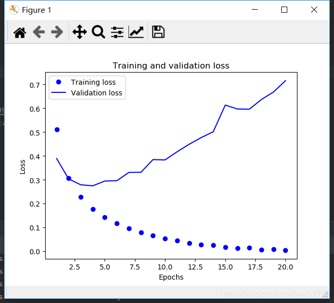
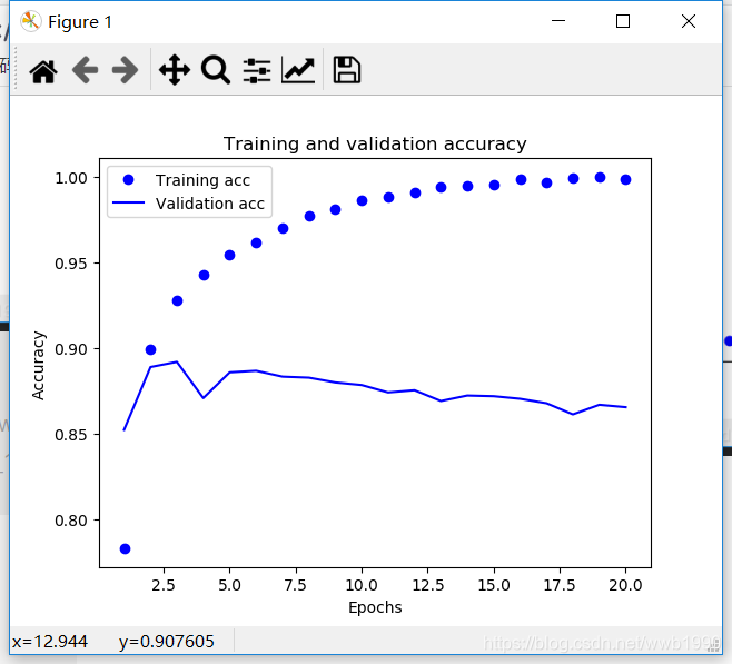可以看出训练损失持续降低，训练精度持续增长。这满足梯度下降的优化预期。
但是可以看到验证损失和验证精度，可以从图中看到，他们在第三到第四个周期达到了最佳。

总之，在训练数据上表现变好，但是在没有见过的验证数据上表现有变动。这就是过拟合（overfit）。
在第2轮后，对训练数据过度优化，最终学得的结果仅针对训练数据。无法泛华到训练集之外的数据。

就需要一种降低过拟合的方案。在后面的章节再来学习。

这里先用一种粗糙简单的方案。
我们只训练四轮。
修改训练参数epochs=4

#训练模型
history = model.fit(partial_x_train,
                    partial_y_trail,
                    epochs=4,
                    batch_size=512,
                    validation_data=(x_val,y_val))

在调用 fit（） 训练之后添加测试集的测试代码，并输出结果：

result = model.evaluate(x_test,y_test)
print(result)

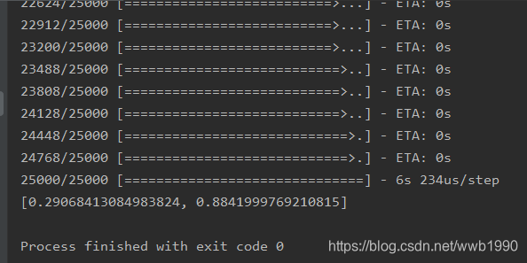
可见这种粗略的策略达到88%的精度。后面再来研究更好的降低过拟合，多做训练的策略。

训练好的网络，使用predict来对评论进行正面的可能性做预测。

predictResult = model.predict(x_test)
print(predictResult)

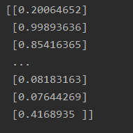
可以看到有非常确定的（>0.99或者<0.01），也有不确信的（0.4~0.6）。

这一节学习就到这。之后可以自行尝试
1.使用1层或者3层隐藏层
2.隐藏单元换成32或者64个
3.用损失函数mse
4.用激活函数tanh

整合上面全部代码：（epochs次数自行修改）

from keras.datasets import imdb
import numpy as np
from keras import models
from keras import layers
import matplotlib.pyplot as plt

(train_data,train_labels),(test_data,test_labels) = imdb.load_data(num_words=10000)
# #第一条评论的单词索引列表
# print(train_data[0])
# #1表示正面品论，0表示负面评论
# print(train_labels[0])
# #取所有测试单词所有的最大的索引值
# print(max([max(sequence) for sequence in train_data]))

# #某条评论解码为英文
# word_index = imdb.get_word_index()
# reverse_word_index = dict(
#     [(value,key) for (key,value) in word_index.items()]
# )
# decoded_review = ' '.join(
#     [reverse_word_index.get(i-3,'?') for i in train_data[0]]
# )
# print(decoded_review)

#转换为10000维的向量，索引的位置是1，其他位置是0
def vectorize_sequences(sequences,dimension=10000):
    results = np.zeros((len(sequences),dimension))
    for i, sequence in enumerate(sequences):
        results[i,sequence] = 1.
    return results
#数据向量化
x_train = vectorize_sequences(train_data)
x_test = vectorize_sequences(test_data)
print(x_train[0])
#标签向量化
y_train = np.asarray(train_labels).astype('float32')
y_test = np.asarray(test_labels).astype('float32')

#模型定义
model = models.Sequential()
model.add(layers.Dense(16,activation='relu',input_shape=(10000,)))
model.add(layers.Dense(16,activation='relu'))
model.add(layers.Dense(1,activation='sigmoid'))
#定义优化器，损失函数，指标
model.compile(optimizer='rmsprop',
              loss='binary_crossentropy',
              metrics=['accuracy'])

#取10000用于验证集
x_val = x_train[:10000] #验证集
partial_x_train = x_train[10000:]

y_val = y_train[:10000] #验证集
partial_y_trail = y_train[10000:]

#训练模型
history = model.fit(partial_x_train,
                    partial_y_trail,
                    epochs=4,
                    batch_size=512,
                    validation_data=(x_val,y_val))

history_dict = history.history
print(history_dict.keys())

loss_values = history_dict['loss']
val_loss_values = history_dict['val_loss']

epochs = range(1,len(loss_values)+1)

plt.plot(epochs,loss_values,'bo',label='Training loss') #bo是蓝色圆点
plt.plot(epochs,val_loss_values,'b',label='Validation loss') #b是蓝色实线
plt.title('Training and validation loss')
plt.xlabel('Epochs')
plt.ylabel('Loss')
plt.legend()
plt.show()

plt.clf() #清空图表

acc_values = history_dict['accuracy']
val_acc_values  = history_dict['val_accuracy']

plt.plot(epochs,acc_values,'bo',label='Training acc') #bo是蓝色圆点
plt.plot(epochs,val_acc_values,'b',label='Validation acc') #b是蓝色实线
plt.title('Training and validation accuracy')
plt.xlabel('Epochs')
plt.ylabel('Accuracy')
plt.legend()
plt.show()

result = model.evaluate(x_test,y_test)
print(result)

predictResult = model.predict(x_test)
print(predictResult)