Pandas & StatsModels 练习题
Reference: http://nbviewer.jupyter.org/github/Schmit/cme193-ipython-notebooks-lecture/tree/master/
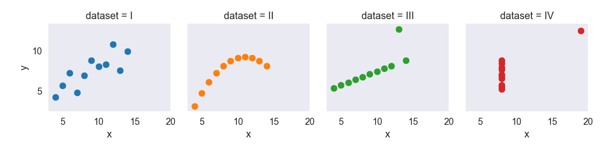
Anscombe’s quartet
Anscombe’s quartet comprises of four datasets, and is rather famous. Why? You’ll find out in this exercise.
import random

import numpy as np
import scipy as sp
import pandas as pd
import matplotlib.pyplot as plt
import seaborn as sns

import statsmodels.api as sm
import statsmodels.formula.api as smf

sns.set_context("talk")
anascombe = pd.read_csv('data/anscombe.csv')
print(anascombe.head())
Output:
  dataset     x     y
0       I  10.0  8.04
1       I   8.0  6.95
2       I  13.0  7.58
3       I   9.0  8.81
4       I  11.0  8.33
Part 1
For each of the four datasets…
- Compute the mean and variance of both and
- Compute the correlation coefficient between and
- Compute the linear regression line: (hint: use statsmodels and look at the Statsmodels notebook)
import random

import numpy as np
import scipy as sp
import pandas as pd
import matplotlib.pyplot as plt
import seaborn as sns

import statsmodels.api as sm
import statsmodels.formula.api as smf

sns.set_context("talk")

anascombe = pd.read_csv('data/anscombe.csv')

print('Mean of x: ')
print(anascombe.groupby('dataset')['x'].mean(), end='\n\n')

print('Variance of x: ')
print(anascombe.groupby('dataset')['x'].var(), end='\n\n')

print('Mean of y: ')
print(anascombe.groupby('dataset')['y'].mean(), end='\n\n')

print('Variance of y: ')
print(anascombe.groupby('dataset')['y'].var(), end='\n\n\n')

print('The correlation coefficient between x and y: ')
print(anascombe.groupby('dataset')[['x', 'y']].corr(), end='\n\n\n')

dataset_groups = anascombe.groupby('dataset')

print('Linear regression: ')
print("Dataset I: ")
lin_model_I = smf.ols('y ~ x', dataset_groups.get_group('I'))
print(lin_model_I.fit().summary(), end='\n\n')

print("Dataset II: ")
lin_model_II = smf.ols('y ~ x', dataset_groups.get_group('II'))
print(lin_model_II.fit().summary(), end='\n\n')

print("Dataset III: ")
lin_model_III = smf.ols('y ~ x', dataset_groups.get_group('III'))
print(lin_model_III.fit().summary(), end='\n\n')

print("Dataset IV: ")
lin_model_IV = smf.ols('y ~ x', dataset_groups.get_group('IV'))
print(lin_model_IV.fit().summary())
Output:
Mean of x:
dataset
I      9.0
II     9.0
III    9.0
IV     9.0
Name: x, dtype: float64

Variance of x:
dataset
I      11.0
II     11.0
III    11.0
IV     11.0
Name: x, dtype: float64

Mean of y:
dataset
I      7.500909
II     7.500909
III    7.500000
IV     7.500909
Name: y, dtype: float64

Variance of y:
dataset
I      4.127269
II     4.127629
III    4.122620
IV     4.123249
Name: y, dtype: float64


The correlation coefficient between x and y:
                  x         y
dataset
I       x  1.000000  0.816421
        y  0.816421  1.000000
II      x  1.000000  0.816237
        y  0.816237  1.000000
III     x  1.000000  0.816287
        y  0.816287  1.000000
IV      x  1.000000  0.816521
        y  0.816521  1.000000


Linear regression:
Dataset I:
                            OLS Regression Results
==============================================================================
Dep. Variable:                      y   R-squared:                       0.667
Model:                            OLS   Adj. R-squared:                  0.629
Method:                 Least Squares   F-statistic:                     17.99
Date:                Fri, 08 Jun 2018   Prob (F-statistic):            0.00217
Time:                        00:28:27   Log-Likelihood:                -16.841
No. Observations:                  11   AIC:                             37.68
Df Residuals:                       9   BIC:                             38.48
Df Model:                           1
Covariance Type:            nonrobust
==============================================================================
                 coef    std err          t      P>|t|      [0.025      0.975]
------------------------------------------------------------------------------
Intercept      3.0001      1.125      2.667      0.026       0.456       5.544
x              0.5001      0.118      4.241      0.002       0.233       0.767
==============================================================================
Omnibus:                        0.082   Durbin-Watson:                   3.212
Prob(Omnibus):                  0.960   Jarque-Bera (JB):                0.289
Skew:                          -0.122   Prob(JB):                        0.865
Kurtosis:                       2.244   Cond. No.                         29.1
==============================================================================

Dataset II:
                            OLS Regression Results
==============================================================================
Dep. Variable:                      y   R-squared:                       0.666
Model:                            OLS   Adj. R-squared:                  0.629
Method:                 Least Squares   F-statistic:                     17.97
Date:                Fri, 08 Jun 2018   Prob (F-statistic):            0.00218
Time:                        00:28:27   Log-Likelihood:                -16.846
No. Observations:                  11   AIC:                             37.69
Df Residuals:                       9   BIC:                             38.49
Df Model:                           1
Covariance Type:            nonrobust
==============================================================================
                 coef    std err          t      P>|t|      [0.025      0.975]
------------------------------------------------------------------------------
Intercept      3.0009      1.125      2.667      0.026       0.455       5.547
x              0.5000      0.118      4.239      0.002       0.233       0.767
==============================================================================
Omnibus:                        1.594   Durbin-Watson:                   2.188
Prob(Omnibus):                  0.451   Jarque-Bera (JB):                1.108
Skew:                          -0.567   Prob(JB):                        0.575
Kurtosis:                       1.936   Cond. No.                         29.1
==============================================================================

Dataset III:
                            OLS Regression Results
==============================================================================
Dep. Variable:                      y   R-squared:                       0.666
Model:                            OLS   Adj. R-squared:                  0.629
Method:                 Least Squares   F-statistic:                     17.97
Date:                Fri, 08 Jun 2018   Prob (F-statistic):            0.00218
Time:                        00:28:27   Log-Likelihood:                -16.838
No. Observations:                  11   AIC:                             37.68
Df Residuals:                       9   BIC:                             38.47
Df Model:                           1
Covariance Type:            nonrobust
==============================================================================
                 coef    std err          t      P>|t|      [0.025      0.975]
------------------------------------------------------------------------------
Intercept      3.0025      1.124      2.670      0.026       0.459       5.546
x              0.4997      0.118      4.239      0.002       0.233       0.766
==============================================================================
Omnibus:                       19.540   Durbin-Watson:                   2.144
Prob(Omnibus):                  0.000   Jarque-Bera (JB):               13.478
Skew:                           2.041   Prob(JB):                      0.00118
Kurtosis:                       6.571   Cond. No.                         29.1
==============================================================================

Dataset IV:
                            OLS Regression Results
==============================================================================
Dep. Variable:                      y   R-squared:                       0.667
Model:                            OLS   Adj. R-squared:                  0.630
Method:                 Least Squares   F-statistic:                     18.00
Date:                Fri, 08 Jun 2018   Prob (F-statistic):            0.00216
Time:                        00:28:27   Log-Likelihood:                -16.833
No. Observations:                  11   AIC:                             37.67
Df Residuals:                       9   BIC:                             38.46
Df Model:                           1
Covariance Type:            nonrobust
==============================================================================
                 coef    std err          t      P>|t|      [0.025      0.975]
------------------------------------------------------------------------------
Intercept      3.0017      1.124      2.671      0.026       0.459       5.544
x              0.4999      0.118      4.243      0.002       0.233       0.766
==============================================================================
Omnibus:                        0.555   Durbin-Watson:                   1.662
Prob(Omnibus):                  0.758   Jarque-Bera (JB):                0.524
Skew:                           0.010   Prob(JB):                        0.769
Kurtosis:                       1.931   Cond. No.                         29.1
==============================================================================
Part 2
Using Seaborn, visualize all four datasets.
hint: use sns.FacetGrid combined with plt.scatter
import pandas as pd

import matplotlib.pyplot as plt
import seaborn as sns

sns.set_style("dark")
sns.set_context("talk")

anascombe = pd.read_csv('data/anscombe.csv')

g = sns.FacetGrid(anascombe, col="dataset", hue="dataset")
g.map(plt.scatter, "x", "y")
plt.show()
Output: