python实现房价预测（一）

这是一个预测房价的项目，项目来自kaggle的housing。

项目的目的是预测房价，需要从众多可能的影响因子中挑选出最能预测房价的因子来建立模型，用于预测房价。

分析步骤：

1. 理解项目目的，再围绕目的进行分析。本项目的目的根据数据预测房价；

2. 了解数据的分布特征，根据实际项目理解每列数据的意义。在数据分析时，最重要的是要熟悉业务，在业务基础上再分析，事半功倍；

3. 挑选特征。刻画每个特征与目标变量之间的关系，找出最重要的特征；同时，为了避免多重共线性，需剔除掉一个特征与特征之间相关性非常大的特征；

4. 应用交叉验证，对训练集进行建立合适的模型，再在测试集上测试；

5. 最终建立预测房价的模型。

下面是实践部分：

1. 首先查看数据

Ask a home buyer to describe their dream house, and they probably won't begin with the height of the basement ceiling or the proximity to an east-west railroad. But this playground competition's dataset proves that much more influences price negotiations than the number of bedrooms or a white-picket fence.

With 79 explanatory variables describing (almost) every aspect of residential homes in Ames, Iowa, this competition challenges you to predict the final price of each home.

SalePrice - the property's sale price in dollars. This is the target variable that you're trying to predict.
MSSubClass: The building class
MSZoning: The general zoning classification
LotFrontage: Linear feet of street connected to property
LotArea: Lot size in square feet
Street: Type of road access
Alley: Type of alley access
LotShape: General shape of property
LandContour: Flatness of the property
Utilities: Type of utilities available
LotConfig: Lot configuration
LandSlope: Slope of property
Neighborhood: Physical locations within Ames city limits
Condition1: Proximity to main road or railroad
Condition2: Proximity to main road or railroad (if a second is present)
BldgType: Type of dwelling
HouseStyle: Style of dwelling
OverallQual: Overall material and finish quality
OverallCond: Overall condition rating
YearBuilt: Original construction date
YearRemodAdd: Remodel date
RoofStyle: Type of roof
RoofMatl: Roof material
Exterior1st: Exterior covering on house
Exterior2nd: Exterior covering on house (if more than one material)
MasVnrType: Masonry veneer type
MasVnrArea: Masonry veneer area in square feet
ExterQual: Exterior material quality
ExterCond: Present condition of the material on the exterior
Foundation: Type of foundation
BsmtQual: Height of the basement
BsmtCond: General condition of the basement
BsmtExposure: Walkout or garden level basement walls
BsmtFinType1: Quality of basement finished area
BsmtFinSF1: Type 1 finished square feet
BsmtFinType2: Quality of second finished area (if present)
BsmtFinSF2: Type 2 finished square feet
BsmtUnfSF: Unfinished square feet of basement area
TotalBsmtSF: Total square feet of basement area
Heating: Type of heating
HeatingQC: Heating quality and condition
CentralAir: Central air conditioning
Electrical: Electrical system
1stFlrSF: First Floor square feet
2ndFlrSF: Second floor square feet
LowQualFinSF: Low quality finished square feet (all floors)
GrLivArea: Above grade (ground) living area square feet
BsmtFullBath: Basement full bathrooms
BsmtHalfBath: Basement half bathrooms
FullBath: Full bathrooms above grade
HalfBath: Half baths above grade
Bedroom: Number of bedrooms above basement level
Kitchen: Number of kitchens
KitchenQual: Kitchen quality
TotRmsAbvGrd: Total rooms above grade (does not include bathrooms)
Functional: Home functionality rating
Fireplaces: Number of fireplaces
FireplaceQu: Fireplace quality
GarageType: Garage location
GarageYrBlt: Year garage was built
GarageFinish: Interior finish of the garage
GarageCars: Size of garage in car capacity
GarageArea: Size of garage in square feet
GarageQual: Garage quality
GarageCond: Garage condition
PavedDrive: Paved driveway
WoodDeckSF: Wood deck area in square feet
OpenPorchSF: Open porch area in square feet
EnclosedPorch: Enclosed porch area in square feet
3SsnPorch: Three season porch area in square feet
ScreenPorch: Screen porch area in square feet
PoolArea: Pool area in square feet
PoolQC: Pool quality
Fence: Fence quality
MiscFeature: Miscellaneous feature not covered in other categories
MiscVal: Value of miscellaneous feature
MoSold: Month Sold
YrSold: Year Sold
SaleType: Type of sale
SaleCondition: Condition of sale

仔细观察每一列特征的含义，以上特征包含建造位置、面积、等级、质量、类型、配套设施、建造时间、出售时间等等。

import numpy as np
import pandas as pd
import seaborn as sns
import matplotlib.pyplot as plt
%matplotlib inline

data = pd.read_csv('train.csv')
# 查看数据
data.head()
# 查看数据集形状
data.shape
# 查看数据集数据类型
data.dtypes

展示部分数据类型，其中包含连续型和离散型数据。

2. 分析目标变量

在分析之前，首先要了解目标，查看目标类型、分布，有无异常值。根据不同的类型选择不同的模型。

[in]: data['SalePrice'].describe()

[out]:

count      1460.000000
mean     180921.195890
std       79442.502883
min       34900.000000
25%      129975.000000
50%      163000.000000
75%      214000.000000
max      755000.000000
Name: SalePrice, dtype: float64

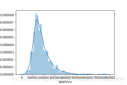
目标变量为连续型，无特别异常值（0或者负数）

再看看目标变量分布：

[in]:sns.distplot(data['SalePrice'])

3. 挑选最佳特征

从80个特征中选出与目标变量SalePrice相关的特征。

a. 针对连续型变量，可以使用“皮尔逊相关系数”找出与目标变量最相关的特征

皮尔逊相关系数是描述两连续性变量线性相关程度的统计量，取值范围[-1,+1]，符号代表相关性正负，数值代表相关性强弱。r=Sxy/(SxSy)

1）一楼面积

sns.jointplot(x='1stFlrSF',y='SalePrice',data=data)

皮尔逊相关系数0.61，中度正相关

2）房屋面积

sns.jointplot(x='GrLivArea',y='SalePrice',data=data)

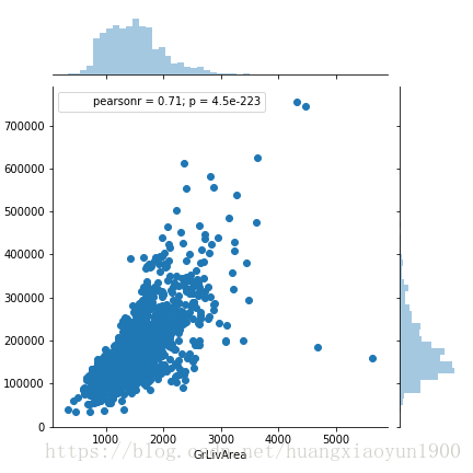
皮尔逊相关系数0.71，强正相关

3）泳池面积

sns.jointplot(x='PoolArea',y='SalePrice',data=data)

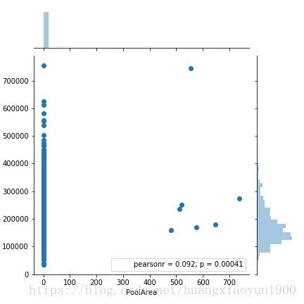
皮尔逊相关系数0.092，不相关

通过以上数据可以看到，建造面积与销售价格有很强的相关性，而一楼面积相关性相对较低，泳池面积几乎无相关性。

相关性越高代表该特征变化能够带来目标变量的变化，需要注意的是相关性并不代表因果关系，只能说特征对目标的影响较大。

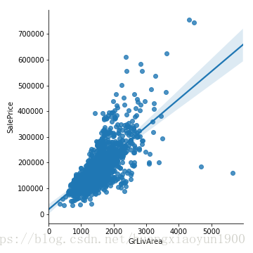
此外，还可以用seaborn里面的线型回归查看拟合直线

sns.lmplot(x='GrLivArea',y='SalePrice',data=data)

b. 针对分类变量，无法使用皮尔逊相关系数，可以通过观察每个分类值上目标变量的变化程度来查看相关性，通常来说，在不同值上数据范围变化较大，两变量相关性较大。

盒须图

1) 房屋材料与质量

sns.boxplot(x='OverallQual',y='SalePrice',data=data)

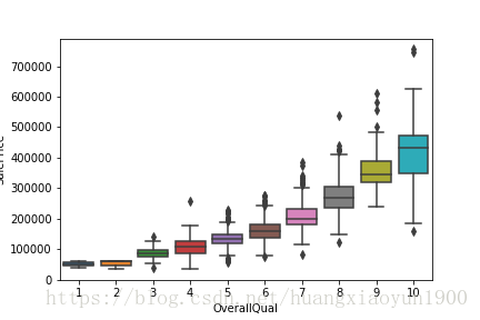
房屋质量越好，总体来说价格越贵

2）建造年代

sns.boxplot(x='YearBuilt',y='SalePrice',data=data)

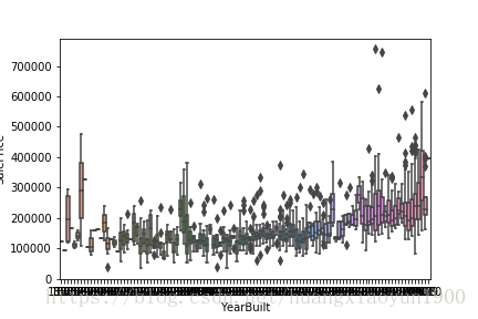
房屋建造年代与价格没有明显的相关性

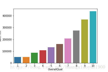
柱状图

使用groupby将价格按照特征分类，再去平均值，使用柱状图展示

grouped = data.groupby('OverallQual')
g1 = grouped['SalePrice'].mean().reset_index('OverallQual')
sns.barplot(x='OverallQual',y='SalePrice',data=g1)

c. 以上两种分析都是针对单个特征与目标变量逐一分析，这种方法非常耗时繁琐，下面介绍一种系统性分析特征与目标变量相关性的方法，通过对数据集整体特征（数值型数据）进行分析，来找出最佳特征。

热力图 sns.heatmap()

首先用计算出两两之间的相关系数data.corr()，再利用热力图显示两两相关性。

%pylab inline
# 设置图幅大小
pylab.rcParams['figure.figsize'] = (15, 10)
# 计算相关系数
corrmatrix = data.corr()
# 绘制热力图，热力图横纵坐标分别是data的index/column,vmax/vmin设置热力图颜色标识上下限，center显示颜色标识中心位置，cmap颜色标识颜色设置
sns.heatmap(corrmatrix,square=True,vmax=1,vmin=-1,center=0.0,cmap='coolwarm')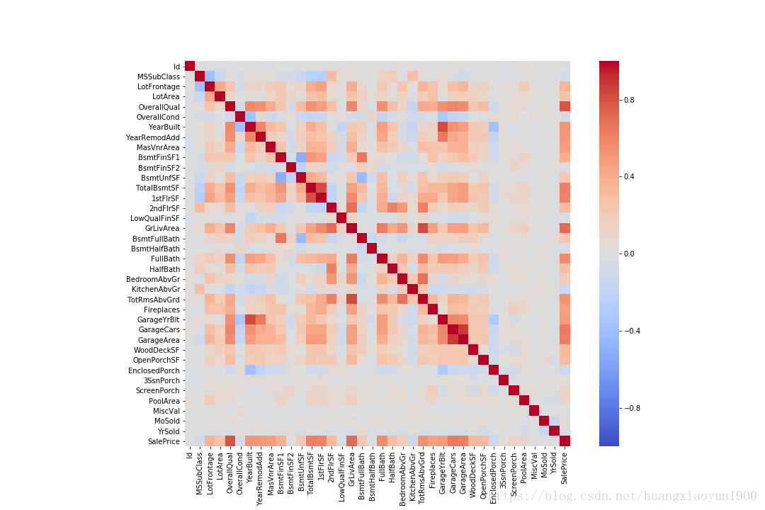

热力图中，不仅可以看到与SalePrice相关性较大的特征，还可以看到与有两个区域相关性比较集中，一个是TotalBsmtSF与1stFlrSF相关性较高，对目标变量来说，这两个特征具有共线性，还有一个是GarageYrBit/GarageCars/GarageArea这三个特征，在建模时，只需去其中一个作为目标变量的特征即可。

特征较多，且相关性不大的特征可以忽略，选取相关性排前十的特征：

# 取相关性前10的特征
k=10
# data.nlargest(k, 'target')在data中取‘target'列值排前十的行
# cols为排前十的行的index,在本例中即为与’SalePrice‘相关性最大的前十个特征名
cols = corrmatrix.nlargest(k,'SalePrice')['SalePrice'].index
cm = np.corrcoef(data[cols].values.T)
#data[cols].values.T
#设置坐标轴字体大小
sns.set(font_scale=1.25)
# sns.heatmap() cbar是否显示颜色条，默认是；cmap显示颜色；annot是否显示每个值，默认不显示；
# square是否正方形方框，默认为False,fmt当显示annotate时annot的格式；annot_kws为annot设置格式
# yticklabels为Y轴刻度标签值，xticklabels为X轴刻度标签值
hm = sns.heatmap(cm,cmap='RdPu',annot=True,square=True,fmt='.2f',annot_kws={'size':10},yticklabels=cols.values,xticklabels=cols.values)


# 上例提供了求相关系数另一种方法，也可以直接用data.corr(),更方便
cm1 = data[cols].corr()
hm2 = sns.heatmap(cm1,square=True,annot=True,cmap='RdPu',fmt='.2f',annot_kws={'size':10})

由上图可以看出：

1. 'OverallQual', 'GrLivArea'这两个变量与'SalePrice'有很强的线性关系;

2. 'GarageCars', 'GarageArea'与'SalePrice'也有很强的线性关系，但'GarageCars', 'GarageArea'相关性0.88，有很强的共线性，只取其一即可，取与目标变量关系更强的'GarageCars'；

3. 同样地，'TotalBsmtSF', '1stFlrSF'也有很强的共线性，只取其一即可，取'TotalBsmtSF'；

4. 因此，选取的特征有：'OverallQual', 'GrLivArea', 'GarageCars', 'TotalBsmtSF', 'FullBath', 'TotRmsAbvGrd', 'YearBuilt'。

sns.pairplot()

cols1 = ['SalePrice', 'OverallQual', 'GrLivArea', 'GarageCars','TotalBsmtSF', 'FullBath', 'TotRmsAbvGrd', 'YearBuilt']
sns.pairplot(data[cols1],size=2.5)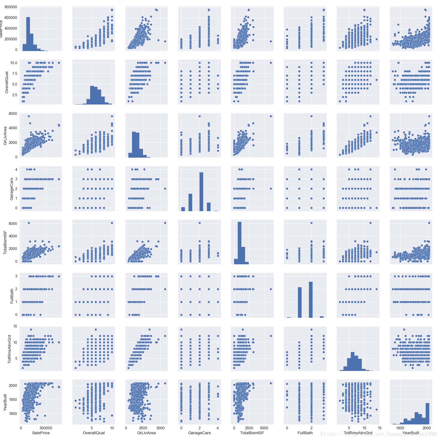

不管是离散型还是连续型数据，只要是数值型数据，sns.heatmap()都能找出两两特征之间的相关性，但要说明的是，这里的离散型数值型特征在处理时被当成连续型特征计算，因此，离散型数值特征的排序会影响相关性结果。

4. 数据处理

a. Missing value

# isnull() boolean, isnull().sum()统计所有缺失值的个数
# isnull().count()统计所有项个数（包括缺失值和非缺失值），.count()统计所有非缺失值个数
total = data.isnull().sum().sort_values(ascending=False)
percent = (data.isnull().sum()/data.isnull().count()).sort_values(ascending=False)
# pd.concat() axis=0 index,axis=1 column, keys列名
missing_data = pd.concat([total,percent],axis=1,keys = ['Total','Percent'])
missing_data.head(20)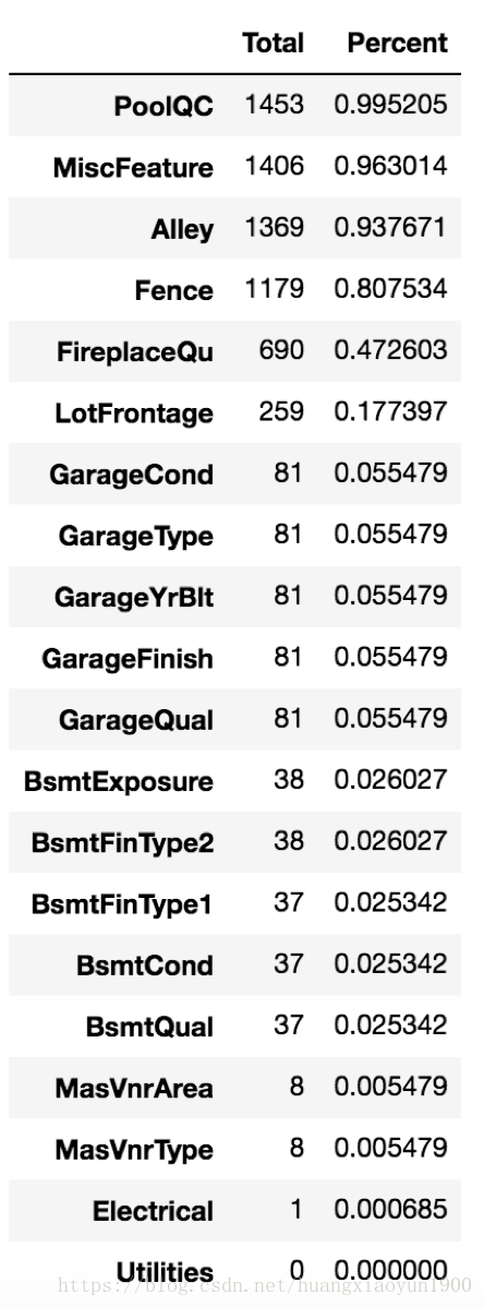

缺失值超过80%的有特征“PoolQC”, "MiscFeature", "Alley", "Fence"，可以认定这些特征无效，可以剔除。

# 处理缺失值，将含缺失值的整列剔除
data1 = data.drop(missing_data[missing_data['Total']>1].index,axis=1)
# 由于特征Electrical只有一个缺失值，故只需删除该行即可
data2 = data1.drop(data1.loc[data1['Electrical'].isnull()].index)
# 检查缺失值数量
data2.isnull().sum().max()

5. 建立模型

首先划分数据集，使用sklearn里面的train_test_split()可以将数据集划分为训练集和测试集。

feature_data = data2.drop(['SalePrice'],axis=1)
target_data = data2['SalePrice']

# 将数据集划分为训练集和测试集
from sklearn.model_selection import train_test_split
X_train,X_test,y_train, y_test = train_test_split(feature_data, target_data, test_size=0.3)

a. 线性回归模型

线性回归模型是最简单的模型，实际应用中已经很少用到了，作为基础知识练习

from statsmodels.formula.api import ols
from statsmodels.sandbox.regression.predstd import wls_prediction_std

df_train = pd.concat([X_train,y_train],axis=1)
# ols("target~feature+C(feature)", data=data
# C(feature)表示这个特征为分类特征category
lr_model = ols("SalePrice~C(OverallQual)+GrLivArea+C(GarageCars)+TotalBsmtSF+C(FullBath)+YearBuilt",data=df_train).fit()
print(lr_model.summary())

# 预测测试集
lr_model.predict(X_test)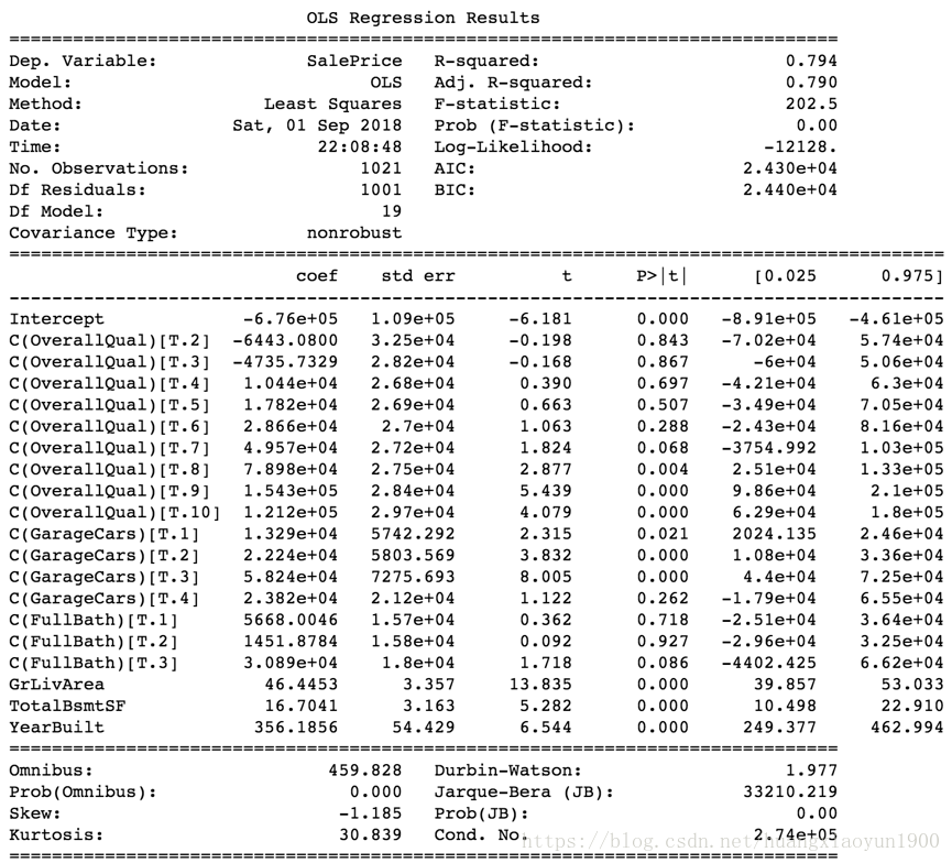

判定系数R2表示，房价“SalePrice”的变异性的79%，能用该多元线性回归方程解释；

在该多元线性回归方程中，也有很多特征的P_value大于0.05，说明这些特征对y值影响非常小，可以剔除。

# prstd为标准方差，iv_l为置信区间下限，iv_u为置信区间上限
prstd, iv_l, iv_u = wls_prediction_std(lr_model, alpha = 0.05)
# lr_model.predict()为训练集的预测值
predict_low_upper = pd.DataFrame([lr_model.predict(),iv_l, iv_u],index=['PredictSalePrice','iv_l','iv_u']).T
predict_low_upper.plot(kind='hist',alpha=0.4)

除了得到模型外，还可以看看模型预测值是否在置信区间之内：wls_prediction_std(model, alpha=0.05)可以得到显著性水平为0.05的置信区间。由以上直方图可以看到预测值均在置信区间内。

虽然线性回归模型能解释79%的房价，但仍然是比较简易基础的模型，接下来会使用更高级的模型对房价进行预测。