转载地址:http://blog.csdn.net/shanglianlm/article/details/46755239
本博文主要讨论 基本矩阵(Basic MF),非负矩阵(Non-negative MF)和正交非负矩阵(Orthogonal non-negative MF)三种常见的矩阵分解方法。并分别推导了它们的更新规则,收敛性,以及它们的应用。
1. 简介(Introduction)
矩阵分解 matrix factorization (MF)
属性(properties)
MF的几个属性:
- 发现数据中的潜在结构 ;
- 它有一个优雅的概率解释(probabilistic interpretation);
- 容易扩展到一些指定特定先验信息的领域 ;
- 许多优化方法例如梯度下降法可以用来找到一个最优解。
三种类型(variants )
该文主要回顾三种矩阵的分解:
- 基本矩阵(Basic MF)
- 非负矩阵(Non-negative MF)
- 正交非负矩阵(Orthogonal non-negative MF)
主要内容
对于每个模型,作者讨论了它的应用场景(the application scenarios),独特属性(the distinctive properties)以及优化方法(the optimizing method)。同时推导了各自的更新规则(updating rules),并证明了它们的正确性和收敛性。最后扩展了它的应用。
2. 理论(Theory)
2.1 基本矩阵(Basic MF)

其中,L(U,V) 是一个用来防止过拟合的正则化项。
Regularization is usually necessary in prediction for bias-variance trade-off [4].
2.1.1 梯度下降算法(Gradient Descent Optimization)
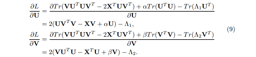
实例化(1),有

The reason of using Frobenius Norm is that it has a Guassian noise interpretation, and that the objective function can be easily transformed to a matrix trace version:
这里写图片描述

note: 这里使用了公式 ||A||F=Tr(ATA)−−−−−−−√ 。迹有很多特点,如Tr(A)=Tr(AT)和Tr(AB)=Tr(BA)。
通过迹导数
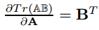
和公式
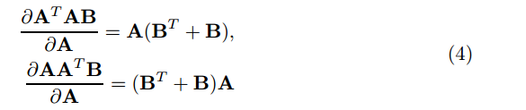
我们有:
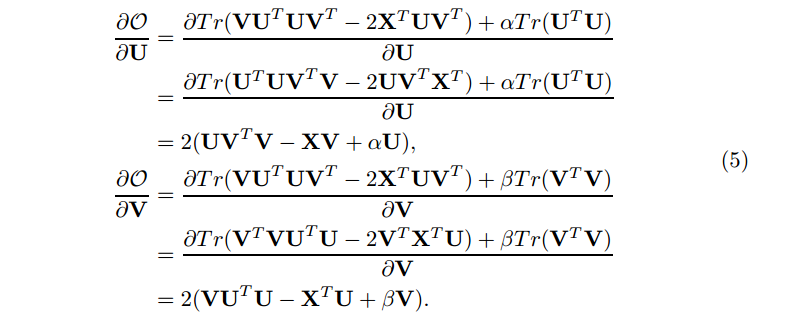
使用这两个导数,我们可以在梯度下降法的每次迭代中交替地更新U和V。
2.2 非负矩阵(Non-negative MF)
非负矩阵分解[13]要求分解获得的矩阵所有项非负,即

除了发现部分外,非负矩阵分解有它自己的计算优势:有一个相对固定的方法来找到一个比一般梯度方法大的学习率(There is a relatively fixed method to find a learning rate larger than common gradient-based methods)。
2.2.1 更新规则推导(Updating Rule Derivation)
基本思路是利用KKT互补松弛条件(complementary slackness conditions)实施非负约束。
(6)式的拉格朗日函数为

我们有下面的KKT条件

其中 ◦ 表示Hadamard 积。接着我们有
令和作为另一个KKT条件,我们有

合并(8)和(10),有

所以我们获得最后的更新规则
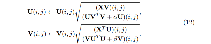
等式(12)直接提供更快收敛的更新规则,不要求手动设定学习率。
2.2.2 收敛性证明(Proof of Convergence)
2.3 正交非负矩阵(Orthogonal non-negative MF)

注意:这里由于正交化的约束,因此没有添加正则化项。
在[5]中,作者证明这个问题等价于k-means聚类。
也可以叫做1-sided 2-factor orthogonal non-negative MF。
2.3.1 三因子矩阵分解和两因子矩阵分解(3-factor MF vs. 2-factor MF)
同时聚类X的行和列,我们需要 3-factor bi-orthogonal non-negative MF

和受限制的1-sided 2-factor orthogonal non-negative MF相比,3-factor bi-orthogonal non-negative MF 能产生更好的近似[5]。
2.3.2 更新规则推导(Updating Rule Derivation)
(24)式的拉格朗日函数为

A. H 的计算(Computation of H)
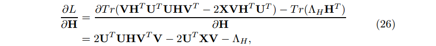
我们有下列KKT条件:
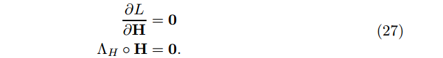
合并上面三个等式,有

因此,我们忽略H的更新规则

注意:推导过程中 UTU≠I。
B. U 和 V 的计算(Computation of U, V)
由于正交约束,求 U 和 V 的更新规则时要求在最后的更新规则中同时消去 Λ 和 Γ 。
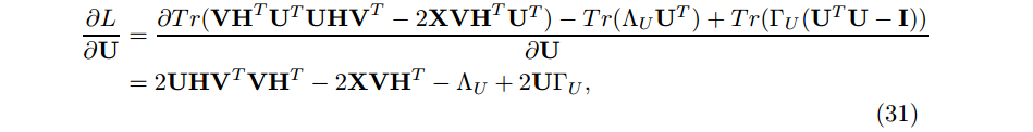
我们有下面的KKT条件:

合并上面三个等式,有

和

注意:这里我们为了获得 ΓU 的一个表达式,因此有 UTU=I。
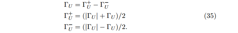
此外,对于 Λ,我们有约束 Λ>0;但是对于 $Γ ,我们没有这个约束。因此我们把切割成两部分,
使用这种划分,我们重写(33)式为

因此 U 最后的更新规则为

类此,V的更新规则为

其中

Choice of 2/3-factor MF How do we choose between 2-factor or 3-factor MF in real-world applications? A general principle is that: if we only need to place regularizations on one latent matrix, i.e. either U or V, then we can use 2-factor MF; if both U and V are to be regularized, either explictly or implictly, 3-factor MF might be a better choice.
3. 关联和应用(Adapatations and Applications)
3.1 稀疏矩阵填充(Sparse Matrix Completion)
这一部分我们主要处理 collborative filtering, link prediction 和 clustering 中的矩阵分解问题。这里我们有一个假设:矩阵中高比例的数据项是缺失的。因此我们形成下面问题

其中 O 是指示矩阵,表明哪项是缺失的。因此目标函数为
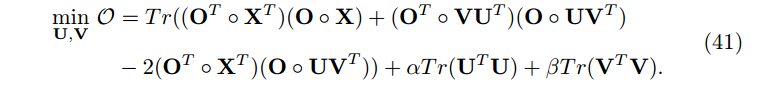
梯度为
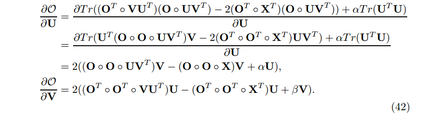
在上面的推导中,我们使用了下面 Hadamard product 的规则

3.1.1 计算内存占用(Calculating Memory Occupation)
对于上面纯 matrix-wise 的更新规则,在实际运算中,可能会溢出内存,可能不如随机梯度下降法(stochasitc gradient descent algorithm )有效。
假如我们有一个 10K × 10K 的矩阵,矩阵每项为一个 30bit 的浮点型数值。那么它的内存分配为 (10^{4} × 10^{4} × 4)/10^{6} = 400M。
3.2 增强矩阵填充(Enhanced Matrix Completion)
这一部分主要考虑当外在数据源可利用的时候的正则化类型。如:
1. self-regularization when we have additional linked data between users (in collaborative filtering (CF), or addtional link type in link prediction (LP)) [6] ;
2. 2-sided regularization when we have description data of users and items [7].
3.2.1 带自正则化的增强矩阵填充(Enhancing Matrix Completion with Self-regularization)
关于 Self-regularization, 我们主要涉及 低秩矩阵 U或V中行的正则化。
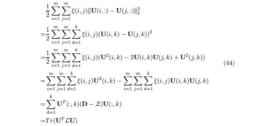
在实际应用中,除了给出的数据外,我们还会有一些其他信息可以利用,关键在于咋样把这些信息加入到应用中,即添加正则化项到目标函数中。例如添加等式(44)到一般的矩阵分解框架中,其中 ξ 是additional link matrix ξ, 对角矩阵 D 的项 D(i,i)=\ximj=1(j,i),因此 L 是 D 和Laplacian 矩阵。
Regularization and Sparseness More regularization sometimes can conquer the data sparsity problem, to some extent. On the other hand, modelling the error only on observed data entries, as what O does in previous subsection, could be also very effective.
3.2.2 带两边正规化的增强矩阵填充(Enhancing Matrix Completion with 2-sided regularization)
这一部分我们考虑对 U 和 V 一起正则化,我们称作 2-sided 正则化。
Regularization, differing from constraints, however can be viewed as a soft type of constraints: it only needs to be satisfied to some extend, while constraints need to be strictly satisified. This is the reason why we consider non-negativity and orthogonality constraints, while call homophily regularization.
[7] 考虑 基于位置的社交网络(location-based social network (LBSN))中的 POI 推荐问题。我们有包含用户和POI交互信息的 登记(check-in)数据 X, 以及关于用户兴趣的描述数据 A 和 关于 POI属性的描述数据 B。问题是怎样利用 A 和 B 增强 交互矩阵(interacting matrix) X 的矩阵填充问题。
因为我们处理的是 2-sided 正则化,因此我们使用 3-factor MF:

问题来了,我们咋样像添加正交化约束那样添加 2-sided 正则化项 R’s ?
为了利用 A 和 B, 我们假设它们之间存在一些联系,即他们 可以用来正则化 U 和 V。在LBSN中,我们可以假设它们有相似的词汇表,即相似的潜在空间。因此,我们可以使用2-factor MF来近似 A 和 B :

其中有关系

等式(47)建立起 U 和 V 之间的关系,形成一个 2-sided 正则化。
最后的目标函数为
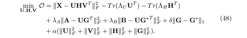
注意:这里我们使用正则化(而不是正交非负矩阵分解中的约束),因此我们可以添加 U, V 和 H 的正则化。
Factorization vs. Regularization We remark here that the idea of cofactoring two matrices (X, A) with shared factors (U) originates from collective matrix facterization , which has many applications in CF . A interesting comparative study between collective facterization and self-regularization can be found in [10].
3.3 从聚类到半监督学习(From Clustering to (Semi-)supervised Learning)
(半)监督学习中使用MF的一个基本假设是对一些响应(response),潜在的行或列是可预测的。为了利用这种预测能力,我们需要一个机制来连接潜在的向量和响应(response)。我们主要考虑下面两种类型:
1. reinforcement directly enforce the latent space to be the response space [8];
2. transformation transform the latent space to response space [9]. This is similar as what people do in machine learning.
参考及延伸阅读材料
[1] Notes on Low-rank Matrix Factorization
[2] Mike Brookes. The matrix reference manual. Imperial College London, 2005.
[3] Chris Ding, Xiaofeng He, and Horst D Simon. On the equivalence of nonnegative matrix factorization and spectral clustering. In SDM’05, pages 606–610. SIAM, 2005.
[4] Trevor Hastie, Robert Tibshirani, and Jerome Friedman. The elements of statistical learning. Springer, 2009.
[5] Chris Ding, Tao Li, Wei Peng, and Haesun Park. Orthogonal nonnegative matrix t-factorizations for clustering. In KDD’06, pages 126–135. ACM, 2006.
[6] Jiliang Tang, Huiji Gao, Xia Hu, and Huan Liu. Exploiting homophily effect for trust prediction. In WSDM’13, pages 53–62. ACM, 2013.
[7] Huiji Gao, Jiliang Tang, Xia Hu, and Huan Liu. Content-aware point of interest recommendation on location-based social networks. In AAAI’15, 2015.
[8] Xia Hu, Jiliang Tang, Huiji Gao, and Huan Liu. Unsupervised sentiment analysis with emotional signals. In WWW’13, pages 607–618. ACM, 2013.
[9] Huiji Gao, Jalal Mahmud, Jilin Chen, Jeffrey Nichols, and Michelle Zhou. Modeling user attitude toward controversial topics in online social media. In ICWSM’14, 2014.
[10] Quan Yuan, Li Chen, and Shiwan Zhao. Factorization vs. regularization: fusing heterogeneous social relationships in top-n recommendation. In Recsys’11, pages 245–252. ACM, 2011.