根据师兄的建议看了resnet论文,又看了一些论文笔记:
https://blog.csdn.net/xxy0118/article/details/78324256
https://blog.csdn.net/lanran2/article/details/79057994
对应之前deeplearning课程完成过的代码再次梳理一遍吧。。。
论文中针对“退化”问题,即随着网络深度增加,准确率变得饱和(这一点在意料之中)随后迅速衰退这一问题,提出了残差网络。
作业中是这么说的:

作业中提到了梯度消失(爆炸)问题,但似乎在这里没有提到标准化的问题,似乎在此将梯度消失全部归因于没有使用resnet。但是反观论文在写作之初是这么说的:

回答这个问题的一个障碍是众所周知的“梯度消失/爆炸”,这阻碍了从一开始就收敛。然而,这个问题主要通过规范化的初始化和中间的标准化层(Batch Normalization)来解决,这使得具有数十层的网络通过随机梯度下降(SGD)方法可以开始收敛。
也就是说这个问题可以用标准化解决,但作业中只将其归因于没有使用ResNet?我能力有限,不知道我这里有没有理解错,暂且放在这里吧。

对于为何使用残差块,论文中在第二部分related work中如此解释:
-------------------------------------------------------------------------------------------------------------------------------------------------------------
残差表达
在图像识别中,VLAD是一种由残差向量关于字典的编码表示,而Fisher Vector可以被定义为VLAD的概率版本。它们都是图像检索和分类的强大的浅层表示。对于向量化,编码残差向量比编码原始向量更有效。
在低层次的视觉和计算机图形学中,为了解决偏微分方程(PDEs),被广泛使用的多网格法将系统重新设计成多个尺度下的子问题,每个子问题负责一个较粗的和更细的尺度之间的残差解。多网格的另一种选择是分层基础的预处理,它依赖于在两个尺度之间表示残差向量的变量。研究表明,这些(转化成多个不同尺度的子问题,求残差解的)解决方案的收敛速度远远快于那些不知道残差的标准解决方案。这些方法表明,良好的重构或预处理可以简化优化问题。
Shortcut Connections
与我们的工作同时,HighwayNetworks提供了与门控功能的shortcut connection。这些门是数据相关的,并且有参数,这与我们的恒等shortcut connection是无参数的。当一个封闭的shortcut connection被关闭(接近于零)时,highway networks中的层代表了无残差的函数。相反,我们的公式总是学习残差函数;我们的恒等shortcut connection永远不会关闭,在学习其他残差函数的同时,所有的信息都会被传递。此外,highway networks还没有显示出从增加深度而获得的准确率的增长(例如:,超过100层)。
------------------------------------------------------------------------------------------------------------------------------------------------------------------
储备知识不够这里看得云里雾里的,查阅了一下关于残差的资料:
---------------------------------------------------------------------------------------------------------------------------------------------------------------------
残差在数理统计中是指实际观察值与估计值(拟合值)之间的差。“残差”蕴含了有关模型基本假设的重要信息。如果回归模型正确的话, 我们可以将残差看作误差的观测值。它应符合模型的假设条件,且具有误差的一些性质。利用残差所提供的信息,来考察模型假设的合理性及数据的可靠性称为残差分析。

在回归分析中,测定值与按回归方程预测的值之差,以δ表示。残差δ遵从正态分布N(0,σ2)。(δ-残差的均值)/残差的标准差,称为标准化残差,以δ*表示。δ*遵从标准正态分布N(0,1)。实验点的标准化残差落在(-2,2)区间以外的概率≤0.05。若某一实验点的标准化残差落在(-2,2)区间以外,可在95%置信度将其判为异常实验点,不参与回归直线拟合。
显然,有多少对数据,就有多少个残差。残差分析就是通过残差所提供的信息,分析出数据的可靠性、周期性或其它干扰。
-------------------------------------------------------------------------------------------------------------------------------------------------------------------
作者对于残差块的介绍:

对于为什么残差网络表现更好,吴恩达给出的解释:

如果网络已经达到最优,继续加深网络,residual mapping被push为0,只剩下identity maping,所以网络性能不会随深度增加而降低。而一般的,多出来的网络结构会学习到一些有用的信息,因此性能可能会更好。
作业中也有提及:
这是包含恒等shortcut的block:


def identity_block(X, f, filters, stage, block):
    """
    Implementation of the identity block as defined in Figure 3

    Arguments:
    X -- input tensor of shape (m, n_H_prev, n_W_prev, n_C_prev)
    f -- integer, specifying the shape of the middle CONV's window for the main path
    filters -- python list of integers, defining the number of filters in the CONV layers of the main path
    stage -- integer, used to name the layers, depending on their position in the network
    block -- string/character, used to name the layers, depending on their position in the network

    Returns:
    X -- output of the identity block, tensor of shape (n_H, n_W, n_C)
    """

    # defining name basis
    conv_name_base = 'res' + str(stage) + block + '_branch'
    bn_name_base = 'bn' + str(stage) + block + '_branch'

    # Retrieve Filters
    F1, F2, F3 = filters

    # Save the input value. You'll need this later to add back to the main path.
    X_shortcut = X

    # First component of main path
    X = Conv2D(filters = F1, kernel_size = (1, 1), strides = (1,1), padding = 'valid', name = conv_name_base + '2a', kernel_initializer = glorot_uniform(seed=0))(X)
    X = BatchNormalization(axis = 3, name = bn_name_base + '2a')(X)
    X = Activation('relu')(X)

    ### START CODE HERE ###

    # Second component of main path (≈3 lines)
    X = Conv2D(filters = F2, kernel_size = (f, f), strides = (1,1), padding = 'same', name = conv_name_base + '2b', kernel_initializer = glorot_uniform(seed=0))(X)
    X = BatchNormalization(axis = 3, name = bn_name_base + '2b')(X)
    X = Activation('relu')(X)

    # Third component of main path (≈2 lines)
    X = Conv2D(filters = F3, kernel_size = (1, 1), strides = (1,1), padding = 'valid', name = conv_name_base + '2c', kernel_initializer = glorot_uniform(seed=0))(X)
    X = BatchNormalization(axis = 3, name = bn_name_base + '2c')(X)

    # Final step: Add shortcut value to main path, and pass it through a RELU activation (≈2 lines)
    X = Add()([X_shortcut, X])
    X = Activation('relu')(X)

    ### END CODE HERE ###

    return X
对于论文中提到的输入输出可能不同的情况,给出了2种残差块形式:
A. shortcut使用恒等映射,对增加的维度用0来填充,不引入额外参数;
B. 投影shortcut用于匹配维数(由1×1卷积完成)。
作业中似乎只给出了包含投影shortcut的block:


def convolutional_block(X, f, filters, stage, block, s = 2):
"""
Implementation of the convolutional block as defined in Figure 4
Arguments:
X -- input tensor of shape (m, n_H_prev, n_W_prev, n_C_prev)
f -- integer, specifying the shape of the middle CONV's window for the main path
filters -- python list of integers, defining the number of filters in the CONV layers of the main path
stage -- integer, used to name the layers, depending on their position in the network
block -- string/character, used to name the layers, depending on their position in the network
s -- Integer, specifying the stride to be used
Returns:
X -- output of the convolutional block, tensor of shape (n_H, n_W, n_C)
"""
# defining name basis
conv_name_base = 'res' + str(stage) + block + '_branch'
bn_name_base = 'bn' + str(stage) + block + '_branch'
# Retrieve Filters
F1, F2, F3 = filters
# Save the input value
X_shortcut = X
##### MAIN PATH #####
# First component of main path
X = Conv2D(F1, (1, 1), strides = (s,s), padding ='valid', name = conv_name_base + '2a', kernel_initializer = glorot_uniform(seed=0))(X)
X = BatchNormalization(axis = 3, name = bn_name_base + '2a')(X)
X = Activation('relu')(X)
### START CODE HERE ###
# Second component of main path (≈3 lines)
X = Conv2D(F2, (f, f), strides = (1,1), padding = 'same', name = conv_name_base + '2b', kernel_initializer = glorot_uniform(seed=0))(X)
X = BatchNormalization(axis = 3, name = bn_name_base + '2b')(X)
X = Activation('relu')(X)
# Third component of main path (≈2 lines)
X = Conv2D(F3, (1, 1), strides = (1,1), padding = 'valid', name = conv_name_base + '2c', kernel_initializer = glorot_uniform(seed=0))(X)
X = BatchNormalization(axis = 3, name = bn_name_base + '2c')(X)
##### SHORTCUT PATH #### (≈2 lines)
X_shortcut = Conv2D(F3, (1, 1), strides = (s,s), padding = 'valid', name = conv_name_base + "1", kernel_initializer = glorot_uniform(seed=0))(X_shortcut)
X_shortcut = BatchNormalization(axis = 3, name = bn_name_base + '1')(X_shortcut)
# Final step: Add shortcut value to main path, and pass it through a RELU activation (≈2 lines)
X = Add()([X_shortcut, X])
X = Activation('relu')(X)
### END CODE HERE ###
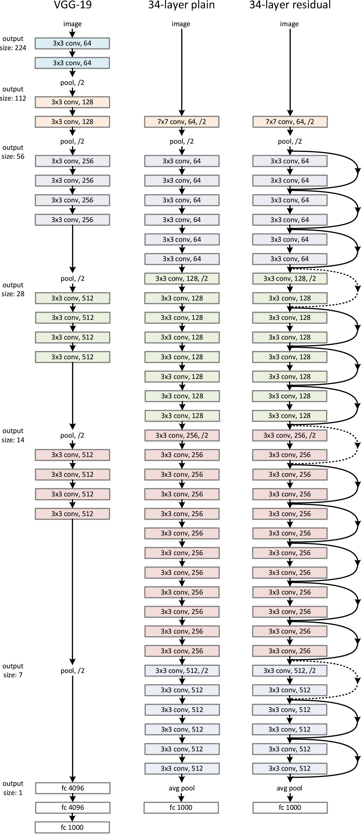
return X在设置由VGG net启发的plain network时,遵循以下原则:
1.对于输出特征图相同的层,拥有相同数量的filter
2.如果特征图大小减半了,filter的数量增倍以保证每层相同的时间复杂度。
在plain network基础上,添加shortcut,有三种方法:
A. 使用恒等映射,如果residual block的输入输出维度不一致,对增加的维度用0来填充;
B. 在block输入输出维度一致时使用恒等映射,不一致时使用线性投影以保证维度一致;
C. 对于所有的block均使用线性投影。
对于三种方法都进行了实验,效果如下:

作者认为,ABC中微小的差别可以说明投影不是必需的。考虑到时间空间复杂度和模型规模,方法C将不再被介绍,而identity shortcut对于不增加bottleneck复杂度有着极其重要的作用。
对于深层bottleneck,如果下图右侧被换成投影shortcut,时间复杂度和模型规模将会加倍,因为shortcut连接了两个高维度端(这一块不太懂。。。先放在这里)

shortcut中间至少跨越有2层因为如果只有一层y=w1*x+x,与线性层很相似,我们就看不到原来的优势了,至于右图的中间一层是bottleneck之前有总结过这里就不赘述了。


对于上表和上图作者提出了三个主要发现:
1.相较于plain-18和plain-34的错误率大小,ResNet取得了相反的结果,更重要的是,ResNet-34取得了可观的相对较低的错误率并且对于验证集更可归纳
2.ResNet-34对于top1 error减少了3.5%,验证了极端深度的网络中残差学习的有效性(怎么感觉和1后半部分说的是一个东西)
3.18层的plain和residual network错误率更相近但ResNet-18收敛更快。说明当网络“不是很深”时,SGD仍能通过plain net找到好的解决方案。
作者在CIFAR-10数据集上验证时,发现1202层residual network表现不如110层,作者认为是过拟合的原因。如果使用maxout和dropout可以获得更好的结果。
