一、认知概念
https://blog.csdn.net/Raoodududu/article/details/82287099
二、 常用结构的tensorflow运用
1. 卷积层
'''通过tf.get_variable的方式创建过滤器的权重变量和偏置变量。'''
#权重变量:前两个维度过滤器尺寸,第三个维度当前层的深度,第四个维度表示过滤器的深度
filter_weight = tf.get_cariable('weights', [5, 5, 3, 16], initializer = tf.truncated_normal_initializer(stddev=0.1))
#偏置变量:过滤器深度
biases = tf.get_variable('biases', [16], initializer=tf.constant_initializer(0.1))

'''卷积层前向传播算法'''
#参数1:输入的节点矩阵[batch, _, _, _];参数2:权重;
#参数3:不同维上的步长[1,_, _, 1],即只对长和宽卷积步长。
#参数4:SAME表示全0填充,VALID表示不添加。
conv = tf.nn.conv2d(input, filter_weight, strides=[1, 1, 1, 1], padding='SAME')
bias = tf.nn.bias_add(conv, biases)
actives_conv = tf.nn.relu(bias)
2.池化层
'''最大池化层的前向传播'''
#参数1:当前层的节点矩阵;参数2:过滤器尺寸[1, _, _, 1]不可跨样例和节点矩阵深度
#参数3,参数4:同上
pool = tf.nn.max_pool(actived_conv, ksize=[1, 5, 5, 1], strides=[1, 2, 2, 1],padding='SAME')
3.区别
卷积层使用过滤器是横跨整个深度,而池化层使用过滤器只影响一个深度节点,所以池化层深度与输入深度相同。
三、经典卷积网络模型
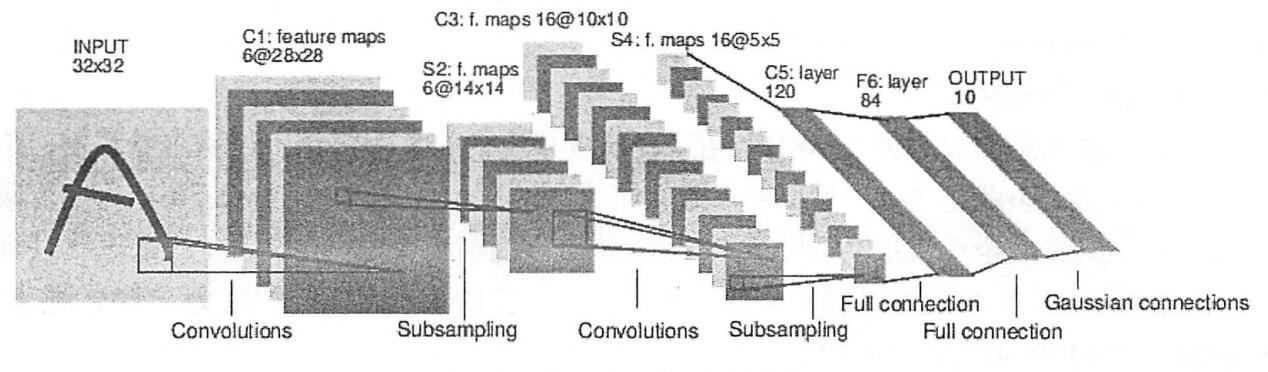
1.LeNet-5模型

优点:大幅提高准确率
缺点:无法很好处理类似ImageNet这样比较大的图像数据集
C1层(卷积层):输入层32×32×1;滤波器尺寸5×5,深度6;不使用全0填充,步长1。
1. 对应特征图大小:特征图的大小28*28,这样能防止输入的连接掉到边界之外(32-5+1=28)。
feature map边长大小的具体计算参见:https://blog.csdn.net/Raoodududu/article/details/82287099
2. 参数个数:C1有156个可训练参数 (每个滤波器5*5=25个unit参数和一个bias参数,一共6个滤波器,共(5*5*1+1)*6=156个参数)
3. 链接个数/FLOPS个数::(28*28)*(5*5+1)*6=122,304个。左边是C1层每个feature map的神经元个数,右边是滤波器在输入层滑过的神经元个数,相乘即为连接数。(每个链接对应1次计算,由wa+b可知,每个参数参与1次计算,所以1个单位的偏置b也算进去)
----------------------------------------
S2层(下采样层):输入层28×28×6;滤波器尺寸2×2;步长2。
1. 对应特征图大小:特征图大小14*14
2. 参数个数:S2层有 12个 (6*(1+1)=12) 可训练参数。S2层 每个滤波器路过的4个邻域 的4个输入相加,乘以1个可训练参数w,再加上1个可训练偏置b(即一个滤波器对应两个参数)。(对于子采样层,每一个特征映射图的的可变参数需要考虑你使用的采样方式而定,如文中的采样方式,每一个特征映射图的可变参数数量为2个,有的采样方式不需要参数)
3. 链接个数/FLOPS个数:5880个连接,( 14*14* (2*2+1)*6 =5880) 。左边是滤波器在C1层滑过的神经元个数,右边是S2层每个feature map的神经元个数,相乘即为连接数。
----------------------------------------
C3层(卷积层):输入层14×14×6;滤波器尺寸5×5,深度16;不使用全0填充,步长1。
1. 对应特征图大小:特征图大小10*10(14-5+1=10)
2. 参数个数:(5×5×6+1)×16
3. 链接个数/FLOPS个数: 10*10*(5×5×6+1)×16=41600个连接。左边是C3层特征图大小,右边是滤波器滑过的S2层神经元个数。
------------------------------------------
S4层(下采样层):输入层10*10*16,;过滤器尺寸2*2,;全0填充,步长2。
1. 对应特征图大小:对应特征图大小5*5。
2. 参数个数:S4层有32个可训练参数。(每个特征图1个因子w和1个偏置b,16*(1+1)=32)
3. 链接个数/FLOPS个数:5*5× (2*2+1)*16 =2000个连接。左边是S4层神经元个数,右边是滤波器在C3层滑过的神经元个数,相乘即为连接数。
--------------------------------------------
C5层(卷积层或第一个全连接层):输入层5*5*16;过滤器尺寸5*5,深度120,步长1。
1. 对应特征图大小:特征图的大小为1*1。(5-5+1=1), 这构成了S4和C5之间的全连接。之所以仍将C5标示为卷积层而非全相联层,是因为如果LeNet-5的输入变大,而其他的保持不变,那么此时特征图的维数就会比1*1大。
2. 参数个数:(16*5*5+1)*120=48120个。滤波器个数120*16个,所以w有120*16*5*5个,同组16个滤波器共用一个b,所以有120个b。
3. 链接个数/FLOPS个数:1*1×48120,左边是C5层特征图大小(其实现在已经变成了单个神经元,大小1*1), 右边是滤波器滑过的神经元个数,相乘即为连接数,此处也即FLOPS个数。
--------------------------------------------
F6层(全连接层):输入120节点,输出84个节点。
1. 对应特征图大小:有84个单元(之所以选这个数字的原因来自于输出层的设计),与C5层全相连。
2. 参数个数:有 84* (120*(1*1)+1)=10164 个可训练参数。如同经典神经网络,F6层计算输入向量(120)和权重向量(1*1)之间的点积,再加上一个偏置(+1)。然后将其传递给sigmoid函数产生单元i的一个状态。
3. 链接个数/FLOPS个数:1*1×10164,左边是F6层特征图大小,右边是滤波器在C5层滑过的神经元个数。
--------------------------------------------
输出层:输入84个节点,输出节点10个。
参数个数:(10+1)×84。
--------------------------------------------

2.LeNet-5代码
(1)inference.py
import tensorflow as tf

# 1.配置参数
INPUT_NODE = 784
OUTPUT_NODE = 10

IMAGE_SIZE = 28
NUM_CHANNELS = 1
NUM_LABELS = 10
# 第一层卷积层的尺寸和深度
CONV1_DEEP = 32
CONV1_SIZE = 5
# 第二层卷积层的尺寸和深度
CONV2_DEEP = 64
CONV2_SIZE = 5
# 全连接层的节点个数
FC_SIZE = 512


# 2.定义前向传播的过程
# 这里添加了一个新的参数train,用于区分训练过程和测试过程。
# 在这个程序中将用到dropout方法,dropout可以进一步提升模型可靠性并防止过拟合
# dropout过程只在训练时使用
def inference(input_tensor, train, regularizer):
    # 定义的卷积层输入为28*28*1的原始MNIST图片像素,使用全0填充后,输出为28*28*32
    with tf.variable_scope('layer1-conv1'):
        conv1_weights = tf.get_variable("weight", [CONV1_SIZE, CONV1_SIZE, NUM_CHANNELS, CONV1_DEEP], initializer=tf.truncated_normal_initializer(stddev=0.1))
        conv1_biases = tf.get_variable("bias", [CONV1_DEEP], initializer=tf.constant_initializer(0.0))
        conv1 = tf.nn.conv2d(input_tensor, conv1_weights, strides=[1, 1, 1, 1], padding='SAME')
        relu1 = tf.nn.relu(tf.nn.bias_add(conv1, conv1_biases))

    # 实现第二层池化层的前向传播过程。这一层输入为14*14*32
    with tf.name_scope('layer2-pool1'):
        pool1 = tf.nn.max_pool(relu1, ksize=[1, 2, 2, 1], strides=[1, 2, 2, 1], padding='SAME')

    # 实现第三层卷积层
    with tf.variable_scope('layer3-conv2'):
        conv2_weights = tf.get_variable("weight", [CONV2_SIZE, CONV2_SIZE, CONV1_DEEP, CONV2_DEEP], initializer=tf.truncated_normal_initializer(stddev=0.1))
        conv2_biases = tf.get_variable("bias", [CONV2_DEEP], initializer=tf.constant_initializer(0.0))
        conv2 = tf.nn.conv2d(pool1, conv2_weights, strides=[1, 1, 1, 1], padding='SAME')
        relu2 = tf.nn.relu(tf.nn.bias_add(conv2, conv2_biases))

    # 实现第四层池化层
    with tf.name_scope('layer4-pool2'):
        pool2 = tf.nn.max_pool(relu2, ksize=[1, 2, 2, 1], strides=[1, 2, 2, 1], padding='SAME')

        # 将第四层池化层的输出转化为第五层全连接的输入格式。
        pool_shape = pool2.get_shape().as_list()                #将矩阵拉直成向量
        nodes = pool_shape[1] * pool_shape[2] * pool_shape[3]   #计算向量长度:即长×宽×深度
        reshaped = tf.reshape(pool2, [pool_shape[0], nodes])    #将第四层输出变成一个batch向量;batch[0]为一个batch中数据的个数。

    # 声明第五层全连接层的变量并实现前向传播过程
    with tf.variable_scope('layer5-fc1'):
        fc1_weights = tf.get_variable("weight", [nodes, FC_SIZE], initializer=tf.truncated_normal_initializer(stddev=0.1))
        if regularizer != None:                     #只有全连接层的权重需要正则化
            tf.add_to_collection('losses', regularizer(fc1_weights))
        fc1_biases = tf.get_variable("bias", [FC_SIZE], initializer=tf.constant_initializer(0.1))
        fc1 = tf.nn.relu(tf.matmul(reshaped, fc1_weights) + fc1_biases)
        if train: fc1 = tf.nn.dropout(fc1, 0.5)    #dropout避免过拟合:在训练时随即将部分节点输出改为0

    # 声明第六层全连接层的变量并实现前向传播过程
    with tf.variable_scope('layer6-fc2'):
        fc2_weights = tf.get_variable("weight", [FC_SIZE, NUM_CHANNELS], initializer=tf.truncated_normal_initializer(stddev=0.1))
        if regularizer != None:
            tf.add_to_collection('losses', regularizer(fc2_weights))
        fc2_biases = tf.get_variable("bias", [NUM_LABELS], initializer=tf.constant_initializer(0.1))
        logit = tf.matmul(fc1, fc2_weights) + fc2_biases
        return logit
(2)train.py
'''mnist_train.'''
import os
import tensorflow as tf
from tensorflow.examples.tutorials.mnist import input_data
import LeNet_5inference as inference
import numpy as np

BATCH_SIZE = 100
LEARNING_RATE_BASE = 0.05
LEARNING_RATE_DECAY = 0.99
REGULARIZATION_RATE = 0.0001
TRAINING_STEPS = 30000
MOVING_AVERAGE_DECAY = 0.99
#模型保存的路径和文件名
MODEL_SAVE_PATH = "D:/python/pycharm/venv/LeNet"
MODEL_NAME = "model.ckpt"

def train(mnist):
    x = tf.placeholder(tf.float32, [BATCH_SIZE, inference.IMAGE_SIZE, inference.IMAGE_SIZE, inference.NUM_CHANNELS], name='x-input')
    y_ = tf.placeholder(tf.float32, [None, inference.OUTPUT_NODE], name='y-input')
    regularizer = tf.contrib.layers.l2_regularizer(REGULARIZATION_RATE)
    y = inference.inference(x, True, regularizer)                                     #前向传播(训练)
    global_step = tf.Variable(0, trainable=False)
    variable_averages = tf.train.ExponentialMovingAverage(MOVING_AVERAGE_DECAY, global_step)
    variables_averages_op = variable_averages.apply(tf.trainable_variables())
    cross_entropy = tf.nn.sparse_softmax_cross_entropy_with_logits(labels=tf.argmax(y_, 1), logits=y)
    cross_entropy_mean = tf.reduce_mean(cross_entropy)
    loss = cross_entropy_mean + tf.add_n(tf.get_collection('losses'))
    learning_rate = tf.train.exponential_decay(LEARNING_RATE_BASE, global_step, mnist.train.num_examples / BATCH_SIZE, LEARNING_RATE_DECAY)
    train_step = tf.train.GradientDescentOptimizer(learning_rate).minimize(loss, global_step=global_step)
    with tf.control_dependencies([train_step, variables_averages_op]):
        train_op = tf.no_op(name='train')
    #初始化TensorFlow持久化类
    saver = tf.train.Saver()
    with tf.Session() as sess:
        tf.initialize_all_variables().run()
        for i in range(5000):
            xs, ys = mnist.train.next_batch(BATCH_SIZE)
            reshaped_xs = np.reshape(xs, (BATCH_SIZE, inference.IMAGE_SIZE, inference.IMAGE_SIZE, inference.NUM_CHANNELS))
            _, loss_value, step = sess.run([train_op, loss, global_step], feed_dict={x: reshaped_xs, y_: ys})
            if i % 1000 == 0:
                 print("After %d training step,loss on training""batch is %g" % (step, loss_value))  #输出当前损失函数的大小
                 #保存当前模型
                 saver.save(sess, os.path.join(MODEL_SAVE_PATH, MODEL_NAME), global_step=global_step)

def main(argv=None):
    mnist = input_data.read_data_sets("D:/python/pycharm/venv/tmp/data", one_hot=True)
    train(mnist)

if __name__ == '__main__':
    tf.app.run()
(3)eval
import time
import math
import tensorflow as tf
import numpy as np
from tensorflow.examples.tutorials.mnist import input_data
import LeNet_5inference as LeNet5_infernece
import LeNet_5train as LeNet5_train

def evaluate(mnist):
    with tf.Graph().as_default() as g:
        # 定义输出为4维矩阵的placeholder
        x = tf.placeholder(tf.float32, [
            mnist.test.num_examples,
            #LeNet5_train.BATCH_SIZE,
            LeNet5_infernece.IMAGE_SIZE,
            LeNet5_infernece.IMAGE_SIZE,
            LeNet5_infernece.NUM_CHANNELS],
                           name='x-input')
        y_ = tf.placeholder(tf.float32, [None, LeNet5_infernece.OUTPUT_NODE], name='y-input')
        validate_feed = {x: mnist.test.images, y_: mnist.test.labels}
        global_step = tf.Variable(0, trainable=False)

        regularizer = tf.contrib.layers.l2_regularizer(LeNet5_train.REGULARIZATION_RATE)
        y = LeNet5_infernece.inference(x, False, regularizer)
        correct_prediction = tf.equal(tf.argmax(y, 1), tf.argmax(y_, 1))
        accuracy = tf.reduce_mean(tf.cast(correct_prediction, tf.float32))

        variable_averages = tf.train.ExponentialMovingAverage(LeNet5_train.MOVING_AVERAGE_DECAY)
        variables_to_restore = variable_averages.variables_to_restore()
        saver = tf.train.Saver(variables_to_restore)

        #n = math.ceil(mnist.test.num_examples / LeNet5_train.BATCH_SIZE)
        n = math.ceil(mnist.test.num_examples / mnist.test.num_examples)
        for i in range(n):
            with tf.Session() as sess:
                ckpt = tf.train.get_checkpoint_state(LeNet5_train.MODEL_SAVE_PATH)
                if ckpt and ckpt.model_checkpoint_path:
                    saver.restore(sess, ckpt.model_checkpoint_path)
                    global_step = ckpt.model_checkpoint_path.split('/')[-1].split('-')[-1]
                    xs, ys = mnist.test.next_batch(mnist.test.num_examples)
                    #xs, ys = mnist.test.next_batch(LeNet5_train.BATCH_SIZE)
                    reshaped_xs = np.reshape(xs, (
                        mnist.test.num_examples,
                        #LeNet5_train.BATCH_SIZE,
                        LeNet5_infernece.IMAGE_SIZE,
                        LeNet5_infernece.IMAGE_SIZE,
                        LeNet5_infernece.NUM_CHANNELS))
                    accuracy_score = sess.run(accuracy, feed_dict={x:reshaped_xs, y_:ys})
                    print("After %s training step(s), test accuracy = %g" % (global_step, accuracy_score))
                else:
                    print('No checkpoint file found')
                    return

# 主程序
def main(argv=None):
    mnist = input_data.read_data_sets("D:/python/pycharm/venv/tmp/data", one_hot=True)
    evaluate(mnist)

if __name__ == '__main__':
    main()
3.可视化
(1)def
import numpy as np
import tensorflow as tf
import matplotlib.pyplot as plt  # plt 用于显示图片
import matplotlib.image as mpimg  # mpimg 用于读取图片
import numpy as np
import LeNet_5inference
import LeNet_5train
from tensorflow.examples.tutorials.mnist import input_data
mnist = input_data.read_data_sets("D:/python/pycharm/venv/tmp/data", one_hot=True)

img1 = mnist.train.images[1]            #1.读入图片2:  (784,)
label1 = mnist.train.labels[1]          #2.读入标签2:  [0. 0. 0. 1. 0. 0. 0. 0. 0. 0.]
print(label1)
print("img_data shape = ", img1.shape)
img1.shape = [28, 28]                   #3.图片转化为28×28矩阵
print(img1.shape)

'''显示图片'''
plt.imshow(img1)                #热度图
plt.show()
plt.imshow(img1, cmap='gray')   #灰度图
plt.show()

'''多张图显示在一张图上'''
plt.subplot(4,8,1)              #4行8列第一个
plt.imshow(img1, cmap='gray')
plt.axis('off')                 #关掉坐标轴
plt.subplot(4,8,9)              #4行8列第九个
plt.imshow(img1, cmap='gray')
plt.axis('off')
plt.show()

'''用测试LeNet_5train'''
# 首先应该把 img1 转为正确的shape (None, 784)
X_img = mnist.train.images[2].reshape([-1, 784])
y_img = mnist.train.labels[2].reshape([-1, 10]) # 这个标签只要维度一致就行了
result = LeNet_5inference.relu1.eval(feed_dict={X_: X_img, y_: y_img})

for _ in xrange(32):
    show_img = result[:,:,:,_]
    show_img.shape = [28, 28]
    plt.subplot(4, 8, _ + 1)
    plt.imshow(show_img, cmap='gray')
    plt.axis('off')
plt.show()
(2)调用
 # 代价函数曲线
    fig1, ax1 = plt.subplots(figsize=(10, 7))
    plt.plot(loss_value)
    ax1.set_xlabel('step')
    ax1.set_ylabel('loss_value')
    plt.title('Cross Loss')
    plt.grid()
    plt.show()
    '''准确率曲线
    fig7, ax7 = plt.subplots(figsize=(10, 7))
    plt.plot(Accuracy)
    ax7.set_xlabel('Epochs')
    ax7.set_ylabel('Accuracy Rate')
    plt.title('Train Accuracy Rate')
    plt.grid()
    plt.show()
    '''
    # ----------------------------------各个层特征可视化-------------------------------
    # imput image
    fig2, ax2 = plt.subplots(figsize=(2, 2))
    ax2.imshow(np.reshape(mnist.train.images[11], (28, 28)))
    plt.show()

    # 第一层的卷积输出的特征图
    input_image = mnist.train.images[11:12]
    conv1_6 = sess.run(inference.relu1, feed_dict={x: input_image})  # [1, 28, 28 ,6]
    conv1_transpose = sess.run(tf.transpose(conv1_6, [3, 0, 1, 2]))
    fig3, ax3 = plt.subplots(nrows=1, ncols=6, figsize=(6, 1))
    for i in range(6):
        ax3[i].imshow(conv1_transpose[i][0])  # tensor的切片[row, column]

    plt.title('Conv1 6x28x28')
    plt.show()

    # 第一层池化后的特征图
    pool1_6 = sess.run(inference.pool1, feed_dict={x: input_image})  # [1, 14, 14, 6]
    pool1_transpose = sess.run(tf.transpose(pool1_6, [3, 0, 1, 2]))
    fig4, ax4 = plt.subplots(nrows=1, ncols=6, figsize=(6, 1))
    for i in range(6):
        ax4[i].imshow(pool1_transpose[i][0])

    plt.title('Pool1 6x14x14')
    plt.show()

    # 第二层卷积输出特征图
    conv2_16 = sess.run(inference.relu2, feed_dict={x: input_image})  # [1, 14, 14, 16]
    conv2_transpose = sess.run(tf.transpose(conv2_16, [3, 0, 1, 2]))
    fig5, ax5 = plt.subplots(nrows=1, ncols=16, figsize=(16, 1))
    for i in range(16):
        ax5[i].imshow(conv2_transpose[i][0])
    plt.title('Conv2 16x14x14')
    plt.show()

    # 第二层池化后的特征图
    pool2_16 = sess.run(inference.pool2, feed_dict={x: input_image})  # [1, 7, 7, 16]
    pool2_transpose = sess.run(tf.transpose(pool2_16, [3, 0, 1, 2]))
    fig6, ax6 = plt.subplots(nrows=1, ncols=16, figsize=(16, 1))
    plt.title('Pool2 16x7x7')
    for i in range(16):
        ax6[i].imshow(pool2_transpose[i][0])

    plt.show()