LeNet-5模型是Yann LeCun教授于1998年在论文Gradient-based learning applied to document recognition中提出的,它是第一个应用于数字识别问题的卷积神经网络。在MNIST数据集上,LeNet-5模型可以达到大约99.2%的正确率。LeNet-5模型总共有7层(不包括输入)。网上有很多关于卷积神经网络的讲解,这里就不细说了,下面主要说一下如何用程序实现LeNet-5模型。可以参考《TensorFlow实战Google深度学习框架》实现类似LeNet-5模型的卷积神经网络结构。
程序主要包括三个部分:mnist_.inference.py、mnist.train.py和mnist.test.py。mnist.inference.py主要定义前向传播的过程以及神经网络中的参数;mnist.train.py定义了LeNet-5模型的训练过程,并保存训练结束后的最终的模型(持久化);mnist.test.py中对测试数据进行测试,计算LeNet模型在MNIST测试集的正确率。
mnist_.inference.py中程序如下:
# -*- coding: utf-8 -*-
import tensorflow as tf

#配置神经网络的参数
INPUT_NODE=784
OUTPUT_NODE=10

IMAGE_SIZE=28
NUM_CHANNELS=1
NUM_LABELS=10

#第一层卷积层的尺寸和深度
CONV1_DEEP=6
CONV1_SIZE=5

#第三层卷积层的尺寸和深度
CONV2_DEEP=16
CONV2_SIZE=5

#第五层卷积层的尺寸和深度
CONV3_DEEP=120
CONV3_SIZE=5

#全连接层的节点个数
FC_SIZE=84


#定义卷积神经网络的前向传播过程。这里添加一个新的参数train,用于区分训练过程和测试过程。在这个程序中将用到Ddropout方法,dropout可以进一步提升模型可靠性
#并防止过拟合,dropout过程只在训练时使用。
def inference(input_tensor,train,regularizer):
	#声明第一层卷积层的变量并实现前向传播过程。通过使用不同的命名空间来隔离不同层的变量,这可以让每一层中的变量命名只需要考虑
	#在当前层的作用,而不需要担心重名的问题。和标准的LeNet-5模型不太一样,这里定义的卷积层输入为28x28x1的原始MNIST图片像素。
	#因为卷积层中使用了全0填充,所以输出为28x28x6的矩阵。
	with tf.variable_scope('layer1-conv1'):
		conv1_weights=tf.get_variable("weight",[CONV1_SIZE,CONV1_SIZE,NUM_CHANNELS,CONV1_DEEP],initializer=tf.truncated_normal_initializer(stddev=0.1))
		conv1_biases=tf.get_variable("bias",[CONV1_DEEP],initializer=tf.constant_initializer(0.0))

		#使用边长为5,深度为6的过滤器,过滤器移动的步长为1,且使用全0填充。
		conv1=tf.nn.conv2d(input_tensor,conv1_weights,strides=[1,1,1,1],padding='SAME')
		relu1=tf.nn.relu(tf.nn.bias_add(conv1,conv1_biases))

	#实现第二层池化层的前向传播过程。这里选用最大池化层,池化层过滤器的边长为2,使用全0填充且移动的步长为2.这一层的输入为上一层的输出
	#也就是28x28x6的矩阵。输出为14x14x6的矩阵。
	with tf.name_scope('layer2-pool1'):
		pool1=tf.nn.max_pool(relu1,ksize=[1,2,2,1],strides=[1,2,2,1],padding='VALID')

	#声明第三层卷积层的变量并实现前向传播过程。这一层输入为14x14x6的矩阵,因为卷积层没有使用全0填充,所以输出为10x10x16的矩阵
	with tf.variable_scope('layer3-conv2'):
		conv2_weights=tf.get_variable("weight",[CONV2_SIZE,CONV2_SIZE,CONV1_DEEP,CONV2_DEEP],initializer=tf.truncated_normal_initializer(stddev=0.1))
		conv2_biases=tf.get_variable("bias",[CONV2_DEEP],initializer=tf.constant_initializer(0.0))

		#使用边长为5,深度为16的过滤器,过滤器移动的步长为1,不使用全0填充
		conv2=tf.nn.conv2d(pool1,conv2_weights,strides=[1,1,1,1],padding='VALID')
		relu2=tf.nn.relu(tf.nn.bias_add(conv2,conv2_biases))

	#实现第四层池化层的前向传播过程。这一层和第二层的结构是一样的。这一层的输入为10x10x16的矩阵,输出为5x5x16的矩阵
	with tf.name_scope('layer4-pool2'):
		pool2=tf.nn.max_pool(relu2,ksize=[1,2,2,1],strides=[1,2,2,1],padding='VALID')

	#声明第五层全连接层(实际上是卷积层)的变量并实现前向传播过程。这一层输入是5x5x16的矩阵,因为没有使用全0填充,
	#所以输出为1x1x120的矩阵
	with tf.name_scope('layer5-conv3'):
		conv3_weights=tf.get_variable("weights",[CONV3_SIZE,CONV3_SIZE,CONV2_DEEP,CONV3_DEEP],initializer=tf.truncated_normal_initializer(stddev=0.1))
		conv3_biases=tf.get_variable("bias",[CONV3_DEEP],initializer=tf.constant_initializer(0.0))
		#使用边长为5,深度为120的过滤器,过滤器移动的步长为1,不使用全0填充
		conv3=tf.nn.conv2d(pool2,conv3_weights,strides=[1,1,1,1],padding='VALID')
		relu3=tf.nn.relu(tf.nn.bias_add(conv3,conv3_biases))

	#将第五层卷积层的输出转化为第六层全连接层的输入格式。第五层的输出为1x1x120的矩阵,然而第六层全连接层需要的输入格式为向量,
	#所以在这里需要将这个1x1x120的矩阵拉直成一个向量。relu3.get_shape函数可以得到第五层输出矩阵的维度而不需要手工计算。注意因为
	#每一层神经网络的输入输出都为一个batch的矩阵,所以这里得到的维度也包含了一个batch中数据的个数。
	pool_shape=relu3.get_shape().as_list()

	#计算将矩阵拉直成向量之后的长度,这个长度就是矩阵长度及深度的乘积。注意这里pool_shape[0]为一个batch中数据的个数。
	nodes=pool_shape[1]*pool_shape[2]*pool_shape[3]
	#通过tf.reshape函数将第五层的输出变成一个batch的向量。
	reshaped=tf.reshape(relu3,[pool_shape[0],nodes])

	#声明第六层全连接层的变量并实现前向传播过程。这一层的输入时拉直之后的一组向量,向量长度为120,输出是一组长度为84的向量
	#这一层和之前在第五章中介绍的基本一致,唯一的区别就是引入了dropout的概念。dropout在训练时会随机将部分节点的输出为改为0.
	#dropout可以避免过拟合问题,从而使得模型在测试数据上的效果更好。dropout一般只在全连接层而不是卷积层或者池化层使用。
	with tf.variable_scope('layer6-fc1'):
		fc1_weights=tf.get_variable("weight",[nodes,FC_SIZE],initializer=tf.truncated_normal_initializer(stddev=0.1))
		#只有全连接层的权重需要加入正则化
		if regularizer !=None:
			tf.add_to_collection('losses',regularizer(fc1_weights))
		fc1_biases=tf.get_variable("bias",[FC_SIZE],initializer=tf.constant_initializer(0.1))
		fc1=tf.nn.relu(tf.matmul(reshaped,fc1_weights)+fc1_biases)
		if train:
			fc1=tf.nn.dropout(fc1,0.5)

	#声明第七层全连接层的变量并实现前向传播过程。这一层的输入为一组长度为84的向量,输出为一组长度为10的向量。这一层的输出通过
	#softmax之后就得到了最后的分类结果。
	with tf.variable_scope('layer7-fc2'):
		fc2_weights=tf.get_variable("weight",[FC_SIZE,NUM_LABELS],initializer=tf.truncated_normal_initializer(stddev=0.1))
		if regularizer !=None:
			tf.add_to_collection('losses',regularizer(fc2_weights))
		fc2_biases=tf.get_variable("bias",[NUM_LABELS],initializer=tf.constant_initializer(0.1))
		logit=tf.matmul(fc1,fc2_weights)+fc2_biases

	#返回第七层的输出
	return logit
mnist_.train.py中程序如下:
# -*- coding: utf-8 -*-
import os
import tensorflow as tf
import numpy as np
from tensorflow.examples.tutorials.mnist import input_data
#加载mnist_interence.py中定义的常量和前向传播函数
import mnist_inference
#配置神经网络的参数
BATCH_SIZE=100
LEARNING_RATE_BASE=0.1
LEARNING_RATE_DECAY=0.99
REGULARAZTION_RATE=0.0001
TRAINING_STEPS=30000
MOVING_AVERAGE_DECAY=0.99
#模型保存的路径和文件名。
MODEL_SAVE_PATH="/model/"
MODEL_NAME="model.ckpt"
#定义训练过程
def train(mnist):
#定义输入输出placeholder,输入为一个四维矩阵
#第一维表示一个batch中样例的个数;第二维和第三维表示图片的尺寸;第四维表示图片的深度
x =tf.placeholder(tf.float32,[BATCH_SIZE,mnist_inference.IMAGE_SIZE,
mnist_inference.IMAGE_SIZE,mnist_inference.NUM_CHANNELS],name="x-input")
y_=tf.placeholder(tf.float32,[None,mnist_inference.OUTPUT_NODE],name="y-input")
regularizer=tf.contrib.layers.l2_regularizer(REGULARAZTION_RATE)
#直接使用mnist_interence.py中定义的前向传播过程
y=mnist_inference.inference(x,True,regularizer)
global_step=tf.Variable(0,trainable=False)
#定义滑动平均类和滑动平均操作
variable_averages=tf.train.ExponentialMovingAverage(MOVING_AVERAGE_DECAY,global_step)
variables_averages_op=variable_averages.apply(tf.trainable_variables())
#定义交叉熵损失
cross_entropy=tf.nn.sparse_softmax_cross_entropy_with_logits(logits=y,labels=tf.argmax(y_,1))
cross_entropy_mean=tf.reduce_mean(cross_entropy)
#定义总损失(交叉熵损失+正则化损失)
loss=cross_entropy_mean+tf.add_n(tf.get_collection('losses'))
#定义学习率
learning_rate=tf.train.exponential_decay(LEARNING_RATE_BASE,global_step,mnist.train.num_examples/BATCH_SIZE,LEARNING_RATE_DECAY)
#定义反向传播算法更新神经网络的参数,同时更新每一个参数的滑动平均值
train_step=tf.train.GradientDescentOptimizer(learning_rate).minimize(loss,global_step=global_step)
with tf.control_dependencies([train_step,variables_averages_op]):
train_op=tf.no_op(name='train')
#检验使用了滑动平均模型的神经网络前向传播的结果是否正确。tf.argmax(average_y,1)计算每一个样例的预测答案。其中average_y是一个
#batch_size*10 的二维数组,每一行表示一个样例的前向传播结果。tf.argmax的第二个参数“1“表示选取最大值的操作尽在第一个维度中进行
#也就是说,只在每一行选取最大值对应的下标。于是得到的结果是一个长度为batch的一维数组,这个一维数组中的值就表示了每一个样例对应的数字识别结果
#tf.equal判断两个张量的每一维是否相等,如果相等返回True,否则返回False。
correct_prediction=tf.equal(tf.argmax(y,1),tf.argmax(y_,1))
#这个运算首先将一个布尔型的数字转换成实数型,然后计算平均值。这个平均值就是模型在这一组数据上的正确率。
accuracy=tf.reduce_mean(tf.cast(correct_prediction,tf.float32))
#初始化Tensorflow持久化类
saver=tf.train.Saver()
with tf.Session() as sess:
#变量初始化
tf.global_variables_initializer().run()
for i in range(TRAINING_STEPS):
xs,ys=mnist.train.next_batch(BATCH_SIZE)
#将输入的训练数据格式调整为一个四维矩阵,并将这个调整后的数据传入sess.run过程
reshaped_xs=np.reshape(xs,(BATCH_SIZE,mnist_inference.IMAGE_SIZE,mnist_inference.IMAGE_SIZE,mnist_inference.NUM_CHANNELS))
_,loss_value,step=sess.run([train_op,loss,global_step],feed_dict={x:reshaped_xs,y_:ys})
#每100轮保存一次模型
if i%1000==0:
#输出当前的训练情况。这里只输出了模型在当前训练patch上的损失函数大小。通过损失函数的大小可以大概了解训练的情况。
#在验证数据集上正确率信息会有一个单独的程序来完成。
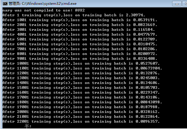
print("Afetr %d training step(s),loss on training batch is %g." % (step,loss_value))
#保存当前的模型。注意这里给出了global_step参数,这样可以让每个被保存模型的文件名末尾加上训练的轮数,比如“model.ckpt-1000”
#表示训练1000轮之后得到的模型。
#saver.save(sess,os.path.join(MODEL_SAVE_PATH,MODEL_NAME),global_step=global_step)
#在测试或者离线时,保存
saver.save(sess,os.path.join(MODEL_SAVE_PATH,MODEL_NAME),global_step=global_step)
#主程序入口
def main(argv=None):
#声明处理MNIST数据集的类,这个类在初始化时会自动下载数据
mnist=input_data.read_data_sets("/tmp/data/",one_hot=True)
train(mnist)
#Tensorflow提供的一个主程序入口,tf.app.run会调用上面定义的main函数。
if __name__ == '__main__':
tf.app.run()
迭代训练过程中总损失变化如下:
mnist_.test.py中程序如下:
# -*- coding: utf-8 -*-
import tensorflow as tf
import numpy as np
from tensorflow.examples.tutorials.mnist import input_data

#加载mnist_inference.py和mnist_train.py 中定义的常量和函数
import mnist_inference
import mnist_train

def evaluate(mnist):
	with tf.Graph().as_default() as g:
		#定义输入输出的格式
		x =tf.placeholder(tf.float32,[mnist.test.num_examples,mnist_inference.IMAGE_SIZE,
			mnist_inference.IMAGE_SIZE,mnist_inference.NUM_CHANNELS],name="x-input")
		y_=tf.placeholder(tf.float32,[None,mnist_inference.OUTPUT_NODE],name="y-input")

		global_step = tf.Variable(0, trainable=False)

		#直接通过调用封装好的函数来计算前向传播结果。因为测试时不关注正则化损失的,所以这里用于计算正则化损失的函数被
		#设置为None,并且train设置为False。
		y=mnist_inference.inference(x,False,None)

		#使用前向传播的结果计算正确率。如果需要对未知样例进行分类,那么使用tf.argmax(y,1)就可以得到输入样例的预测类别了
		correct_prediction=tf.equal(tf.argmax(y,1),tf.argmax(y_,1))
		accuracy=tf.reduce_mean(tf.cast(correct_prediction,tf.float32))

		#通过变量重命名的方式来加载模型,这样在前向传播的过程中就不需要调用求滑动平均的函数来获取平均值了。这样就可以完全共用
		#mnsit_inference.py中定义前向传播过程。
		variable_averages=tf.train.ExponentialMovingAverage(mnist_train.MOVING_AVERAGE_DECAY)
		variables_to_restore=variable_averages.variables_to_restore()
		saver=tf.train.Saver(variables_to_restore)

		with tf.Session() as sess:

			#将输入的测试数据格式调整为一个四维矩阵,并将这个调整后的数据传入sess.run过程
			xs, ys = mnist.test.next_batch(mnist.test.num_examples)
			reshaped_xs=np.reshape(xs,(mnist.test.num_examples,
			                           mnist_inference.IMAGE_SIZE,
									   mnist_inference.IMAGE_SIZE,
									   mnist_inference.NUM_CHANNELS))

			#tf.train.get_checkpoint_state函数会通过cheakpoint文件自动找目录中最新模型的文件名。
			ckpt=tf.train.get_checkpoint_state(mnist_train.MODEL_SAVE_PATH)
			if ckpt and ckpt.model_checkpoint_path:
				#加载模型
				saver.restore(sess,ckpt.model_checkpoint_path)
				#通过文件名得到模型保存时迭代的轮数(训练迭代的总轮数)
				global_step=ckpt.model_checkpoint_path.split('/')[-1].split('-')[-1]
				#计算测试数据分类正确率
				accuracy_test=sess.run(accuracy,feed_dict={x:reshaped_xs, y_:ys})
				#输出测试结果和验证结果
				print("After %s training step(s), test accuracy=%g" % (global_step,accuracy_test))

#主程序入口
def main(argv=None):
	#声明处理MNIST数据集的类,这个类在初始化时会自动下载数据
	mnist=input_data.read_data_sets("/tmp/data/",one_hot=True)
	evaluate(mnist)

#Tensorflow提供的一个主程序入口,tf.app.run会调用上面定义的main函数。
if __name__ == '__main__':
	tf.app.run()
测试结果:
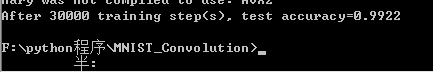
从最终的测试结果中可以看出,LeNet-5模型可以达到大约99.2%的正确率。