内容来自 麦子学院 深度学习基础及介绍
1 神经网络
多层向前神经网络:Multilayer Feed-Forward Neural Network
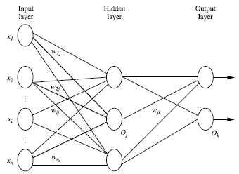
定义:有输入层、隐藏层、输出层,每层由单元组成。输入层由训练集的特征向量传入,经过单元的权重加权求和,作为下一层的输入。如果有足够多的隐藏层,和足够大的训练集,可以模拟出任何方程。
设计结构:确定层数、每层单元数;输入特征向量先要标准化到0~1之间;可以编码离散变量;可用于分类或回归;隐藏层的多少则没有规定,根据经验选取;
交叉验证:在给定的建模样本中,拿出大部分样本进行建模型,留小部分样本用刚建立的模型进行预报,并求这小部分样本的预报误差,记录它们的平方加和。这个过程一直进行,直到所有的样本都被预报了一次而且仅被预报一次。把每个样本的预报误差平方加和,称为PRESS
核心算法:backpropagation:对比预测值与真实值之间的值,反向传播,最小化误差,更新每个连接的权重。初始权重和偏向随机分配。
下面的程序定义了用于神经网络算法的类:
import numpy as np  #科学计算库
def tanh(x):
    return np.tanh(x)
def tanh_deriv(x):
    return 1.0 - np.tanh(x)*np.tanh(x)
def logistic(x):
    return 1/(1 + np.exp(-x))
def logistic_derivative(x):
    return logistic(x)*(1-logistic(x))
class NeuralNetwork:
    def __init__(self, layers, activation='tanh'):
        """
        :param layers: A list containing the number of units in each layer.
        Should be at least two values
        :param activation: The activation function to be used. Can be
        "logistic" or "tanh"
        """
        if activation == 'logistic':
            self.activation = logistic
            self.activation_deriv = logistic_derivative
        elif activation == 'tanh':
            self.activation = tanh
            self.activation_deriv = tanh_deriv
        self.weights = []       #存放权重,初始化时随机产生
        for i in range(1, len(layers) - 1):     #除输出层外均需要初始化
            self.weights.append((2*np.random.random((layers[i - 1] + 1, layers[i] + 1))-1)*0.25)
            self.weights.append((2*np.random.random((layers[i] + 1, layers[i + 1]))-1)*0.25)
    #############################################################################
    def fit(self, X, y, learning_rate=0.2, epochs=10000):# x为训练集,y为标记,学习率,循环次数
        X = np.atleast_2d(X)    #二维
        temp = np.ones([X.shape[0], X.shape[1]+1])  #设定形状
        temp[:, 0:-1] = X  # adding the bias unit to the input layer# 所有行,除去最后一列
        X = temp           #完成bias的添加
        y = np.array(y)    #数据类型转换

        for k in range(epochs):                 #epochs次循环
            i = np.random.randint(X.shape[0])   #每次随机抽取一行
            a = [X[i]]

            for l in range(len(self.weights)):  #going forward network, for each layer
                a.append(self.activation(np.dot(a[l], self.weights[l])))  #Computer the node value for each layer (O_i) using activation function
            error = y[i] - a[-1]  #计算误差
            deltas = [error * self.activation_deriv(a[-1])] #For output layer, Err calculation (delta is updated error)
            #Staring backprobagation 反向更新
            for l in range(len(a) - 2, 0, -1): # 从最后一层开始,每次往回退一层
                #Compute the updated error (i,e, deltas) for each node going from top layer to input layer
                deltas.append(deltas[-1].dot(self.weights[l].T)*self.activation_deriv(a[l]))#更新隐藏层的函数
            deltas.reverse()#逆向传播
            for i in range(len(self.weights)):
                layer = np.atleast_2d(a[i])
                delta = np.atleast_2d(deltas[i])
                self.weights[i] += learning_rate * layer.T.dot(delta) #更新权重的公式
#########################################################################################
    def predict(self, x):
        x = np.array(x)
        temp = np.ones(x.shape[0]+1)
        temp[0:-1] = x
        a = temp
        for l in range(0, len(self.weights)):
            a = self.activation(np.dot(a, self.weights[l]))
        return a
简单测试:
nn = NeuralNetwork( [2,2,1],'tanh' )
X = np.array( [[0,0],[0,1],[1,0],[1,1]] )
y = np.array( [0,1,1,0] )
nn.fit(X,y)
for i in [ [0,0],[0,1],[1,0],[1,1] ]:
    print(i,nn.predict(i))
获得输出:
[0, 0] [0.0027874]
[0, 1] [0.99831001]
[1, 0] [0.99827609]
[1, 1] [-0.01162434]
手写数字识别:
# 每个图片8x8  识别数字:0,1,2,3,4,5,6,7,8,9
import numpy as np
from sklearn.datasets import load_digits    #手写数字的数据集
from sklearn.metrics import confusion_matrix, classification_report #显示预测结果的衡量
from sklearn.preprocessing import LabelBinarizer    #标签二值化
from NeuralNetwork import NeuralNetwork
from sklearn.cross_validation import train_test_split   #拆分数据集
digits = load_digits()
X = digits.data
y = digits.target
X -= X.min()  # normalize the values to bring them into the range 0-1
X /= X.max()
nn = NeuralNetwork([64, 100, 10], 'logistic')   #8*8的像素共64个特征输入,10个数字输出层,隐藏层比输入层多
X_train, X_test, y_train, y_test = train_test_split(X, y)
labels_train = LabelBinarizer().fit_transform(y_train)
labels_test = LabelBinarizer().fit_transform(y_test)
print ("start fitting")
nn.fit(X_train, labels_train, epochs=3000)
predictions = []
for i in range(X_test.shape[0]):
    o = nn.predict(X_test[i])
    predictions.append(np.argmax(o))
print( confusion_matrix(y_test, predictions) )
print( classification_report(y_test, predictions) )
输出结果:
start fitting  #这个矩阵表示预测的结果
[[45  0  0  0  0  0  0  0  0  0]
 [ 0 39  0  0  0  1  0  0  2  2]
 [ 0  3 43  1  0  0  0  0  0  0]
 [ 0  1  0 36  0  1  0  1  2  0]
 [ 0  3  0  0 41  0  0  0  1  0]
 [ 0  0  0  0  1 41  1  0  0  0]
 [ 0  1  0  0  0  0 46  0  0  0]
 [ 0  0  0  0  2  0  0 42  1  2]
 [ 0  2  0  0  0  2  0  0 41  0]
 [ 0  0  0  0  0  0  0  0  3 43]]
             precision    recall  f1-score   support

          0       1.00      1.00      1.00        45
          1       0.80      0.89      0.84        44
          2       1.00      0.91      0.96        47
          3       0.97      0.88      0.92        41
          4       0.93      0.91      0.92        45
          5       0.91      0.95      0.93        43
          6       0.98      0.98      0.98        47
          7       0.98      0.89      0.93        47
          8       0.82      0.91      0.86        45
          9       0.91      0.93      0.92        46

avg / total       0.93      0.93      0.93       450
2 线性回归
回归的变量为连续型数值,分类的变量为离散型数值。
简单线性回归:只有一个因变量和一个自变量;有多个变量时,称为多元回归
简单线性回归示例:
import numpy as np
def fitSLR(x,y):
    n=len(x)
    dinominator = 0
    numerator=0
    for i in range(0,n):
        numerator += (x[i]-np.mean(x))*(y[i]-np.mean(y))
        dinominator += (x[i]-np.mean(x))**2
    print("numerator:"+str(numerator))
    print("dinominator:"+str(dinominator))
    b1 = numerator/float(dinominator)
    b0 = np.mean(y)/float(np.mean(x))
    return b0,b1
# y= b0+x*b1
def prefict(x,b0,b1):
    return b0+x*b1
x=[1,3,2,1,3]
y=[14,24,18,17,27]
b0,b1=fitSLR(x, y)
y_predict = prefict(6,b0,b1)
print("y_predict:"+str(y_predict))
输出:
numerator:20.0
dinominator:4.0
y_predict:40.0
多元回归模型:
from numpy import genfromtxt
from sklearn import linear_model
dataPath = r"Delivery.csv"
deliveryData = genfromtxt(dataPath,delimiter=',')
#print ("data"); print (deliveryData)
x= deliveryData[:,:-1]; y = deliveryData[:,-1]
print ('x=',x); print ('y=',y)
lr = linear_model.LinearRegression()
lr.fit(x, y) ; print (lr)
print("coefficients:"); print (lr.coef_)
print("intercept:"); print (lr.intercept_)
xPredict = [[102,6]]
yPredict = lr.predict(xPredict)
print("predict:"); print (yPredict)
输出:
x= [[100.   4.]
 [ 50.   3.]
 [100.   4.]
 [100.   2.]
 [ 50.   2.]
 [ 80.   2.]
 [ 75.   3.]
 [ 65.   4.]
 [ 90.   3.]
 [ 90.   2.]]
y= [9.3 4.8 8.9 6.5 4.2 6.2 7.4 6.  7.6 6.1]
LinearRegression(copy_X=True, fit_intercept=True, n_jobs=1, normalize=False)
coefficients:
[0.0611346  0.92342537]
intercept:
-0.8687014667817126
predict:
[10.90757981]
非线性回归(逻辑回归)
,其向量式为:
import numpy as np
import random
def genData(numPoints,bias,variance):#创建数据:数据实例(行数),偏好,方差
    x = np.zeros(shape=(numPoints,2))#行,2列
    y = np.zeros(shape=(numPoints))
    for i in range(0,numPoints):
        x[i][0]=1
        x[i][1]=i
        y[i]=(i+bias)+random.uniform(0,1)+variance
    return x,y
def gradientDescent(x,y,theta,alpha,m,numIterations):#梯度下降算法
    xTran = np.transpose(x)
    for i in range(numIterations):
        hypothesis = np.dot(x,theta)
        loss = hypothesis-y
        cost = np.sum(loss**2)/(2*m)
        gradient=np.dot(xTran,loss)/m
        theta = theta-alpha*gradient
        print ("Iteration %d | cost :%f" %(i,cost))
    return theta
x,y = genData(100, 25, 10)
#print ("x:",x); print ("y:",y)
m,n = np.shape(x); n_y = np.shape(y)
print("m:"+str(m)+" n:"+str(n)+" n_y:"+str(n_y))
numIterations = 100000
alpha = 0.0005; theta = np.ones(n)
theta= gradientDescent(x, y, theta, alpha, m, numIterations)
print(theta)
输出:
......
Iteration 99995 | cost :0.042589
Iteration 99996 | cost :0.042589
Iteration 99997 | cost :0.042589
Iteration 99998 | cost :0.042589
Iteration 99999 | cost :0.042589
[35.63312517  0.99751602]