内容来自 麦子学院 深度学习基础及介绍
1 决策树算法:ID3、c4.5、CART
下面是用ID3算法预测的示例:
from sklearn.feature_extraction import DictVectorizer
import csv
from sklearn import tree
from sklearn import preprocessing
from sklearn.externals.six import StringIO
# Read in the csv file and put features into list of dict and list of class label
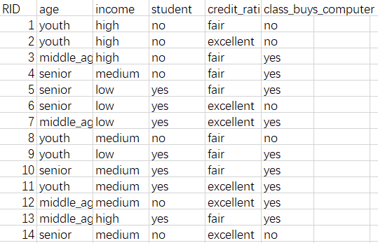
allElectronicsData = open(r'X:\AllElectronics.csv', 'rt') #训练集文件
reader = csv.reader(allElectronicsData)
headers = next(reader)
#print(headers)
featureList = [] #age/income/student/...
labelList = [] #yes or no
for row in reader: #将原始数据转换为列表,包含很多字典
labelList.append(row[len(row)-1])
rowDict = {}
for i in range(1, len(row)-1):
rowDict[headers[i]] = row[i]
featureList.append(rowDict)
#print(featureList);print(labelList)
# Vetorize features
vec = DictVectorizer() #特征向量化、字典特征提取
dummyX = vec.fit_transform(featureList) .toarray() #转换为0-1的格式,有10个特征
#print("dummyX: " + str(dummyX))
#print(vec.get_feature_names())
#print("labelList: " + str(labelList))
# vectorize class labels
lb = preprocessing.LabelBinarizer()
dummyY = lb.fit_transform(labelList)
#print("dummyY: " + str(dummyY))
# Using decision tree for classification
# clf = tree.DecisionTreeClassifier() #默认采用的是CART
clf = tree.DecisionTreeClassifier(criterion='entropy') #信息熵
clf = clf.fit(dummyX, dummyY) #建模,将特征值和标签输入
#print("clf: " + str(clf))
# Visualize model
with open("allElectronicInformationGainOri.dot", 'w') as f: #创建dot文件
f = tree.export_graphviz(clf, feature_names=vec.get_feature_names(), out_file=f)
oneRowX = dummyX[0, :] #读取原数据的第一行
#print("oneRowX: " + str(oneRowX))
newRowX = oneRowX #创建新的一行数据用于预测
newRowX[0] = 1
newRowX[2] = 0
#print("newRowX: " + str(newRowX)) #这时的新数据为[1. 0. 0. 0. 1. 1. 0. 0. 1. 0.]
#print(newRowX.shape) #输出为(10,)
newRowX = newRowX.reshape(1,-1)
#print(newRowX.shape) #输出为(1,10)
predictedY = clf.predict(newRowX)
#print("predictedY: " + str(predictedY)) #预测为1通过Graphviz可视化的图片:
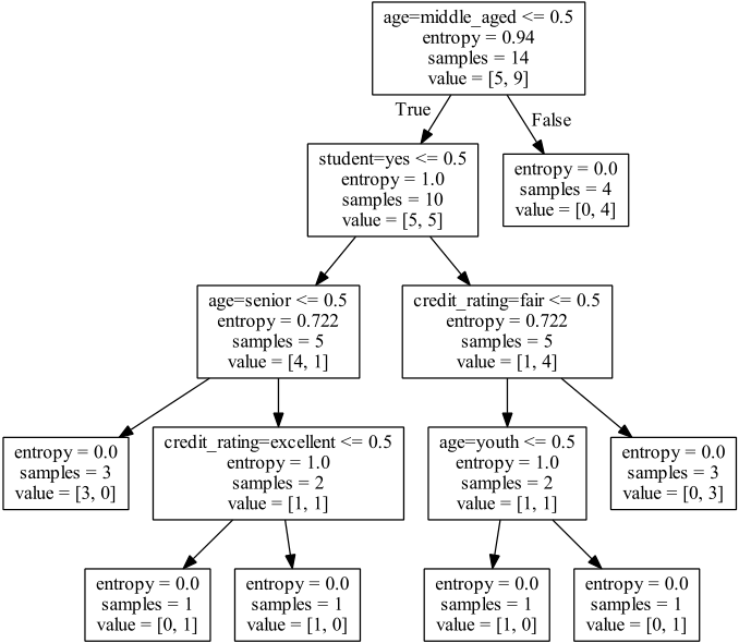
训练集:需要对数据做预处理,将feature和label转换为数值
对age,将其转换为三维向量:分别对应youth\middle\senior,以1-0的形式;共有10维向量表示一个对象的feature。
2 最邻近规则分类KNN算法
使用sklearn模块,以及iris数据集进行建模和预测:
from sklearn import neighbors
from sklearn import datasets
knn = neighbors.KNeighborsClassifier()
iris = datasets.load_iris()
#print(iris)
knn.fit(iris.data,iris.target) #建立模型
predictedLabel = knn.predict([[0.1,0.2,0.3,0.4]])#预测,使用默认参数
print(predictedLabel) #预测输出为[0]
使用代码实现:
import csv
import random
import math
import operator
#装载数据集,参数:(文件名,将文件分界,训练集,测试集)
def loadDataset(filename, split, trainingSet = [], testSet = []):
with open(filename, 'rt') as csvfile:
lines = csv.reader(csvfile) #读取数据
dataset = list(lines) #将数据转换为列表
for x in range(len(dataset)-1):
for y in range(4):
dataset[x][y] = float(dataset[x][y])
if random.random() < split: #随机产生一个值,用以区分训练集和数据集
trainingSet.append(dataset[x])
else:
testSet.append(dataset[x])
#计算欧氏距离,传入两个实例及其深度
def euclideanDistance(instance1, instance2, length):
distance = 0
for x in range(length):
distance += pow((instance1[x]-instance2[x]), 2)
return math.sqrt(distance)
#返回最近的K的点:从训练集中找到k个离这个测试数据最近的点
def getNeighbors(trainingSet, testInstance, k):
distances = []
length = len(testInstance)-1
for x in range(len(trainingSet)):
#testinstance
dist = euclideanDistance(testInstance, trainingSet[x], length)
distances.append((trainingSet[x], dist)) #包含所有点的距离
#distances.append(dist)
distances.sort(key=operator.itemgetter(1)) #从小到大排序
neighbors = []
for x in range(k): #取前k个点
neighbors.append(distances[x][0])
return neighbors
#投票决定输出哪一类
def getResponse(neighbors):
classVotes = {}
for x in range(len(neighbors)):
response = neighbors[x][-1]
if response in classVotes:
classVotes[response] += 1
else:
classVotes[response] = 1
sortedVotes = sorted(classVotes.items(), key=operator.itemgetter(1), reverse=True)
return sortedVotes[0][0] #从大到小排序,返回票数最多的
#预测的准确率
def getAccuracy(testSet, predictions):
correct = 0 #预测正确的个数
for x in range(len(testSet)):
if testSet[x][-1] == predictions[x]:
correct += 1
return (correct/float(len(testSet)))*100.0
#主函数
def main():
#prepare data
trainingSet = []
testSet = []
split = 0.67
loadDataset(r'X:\irisdata.txt', split, trainingSet, testSet)
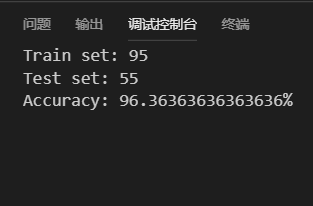
print ('Train set: ' + repr(len(trainingSet)))
print ('Test set: ' + repr(len(testSet)))
#generate predictions
predictions = []
k = 3
for x in range(len(testSet)):
# trainingsettrainingSet[x]
neighbors = getNeighbors(trainingSet, testSet[x], k)
result = getResponse(neighbors)
predictions.append(result)
#print ('>predicted=' + repr(result) + ', actual=' + repr(testSet[x][-1]))
#print ('predictions: ' + repr(predictions))
accuracy = getAccuracy(testSet, predictions)
print('Accuracy: ' + repr(accuracy) + '%')
if __name__ == '__main__':
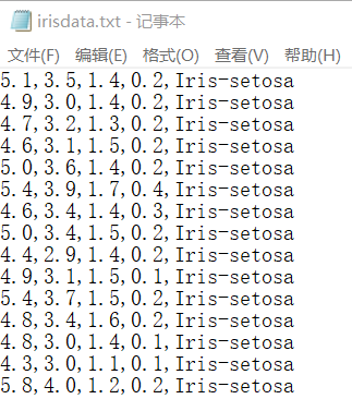
main()其中,irisdata.txt内容如下:包含3类共150个数据,每次根据split = 0.67分出的数据集不等,准确率在90%以上。
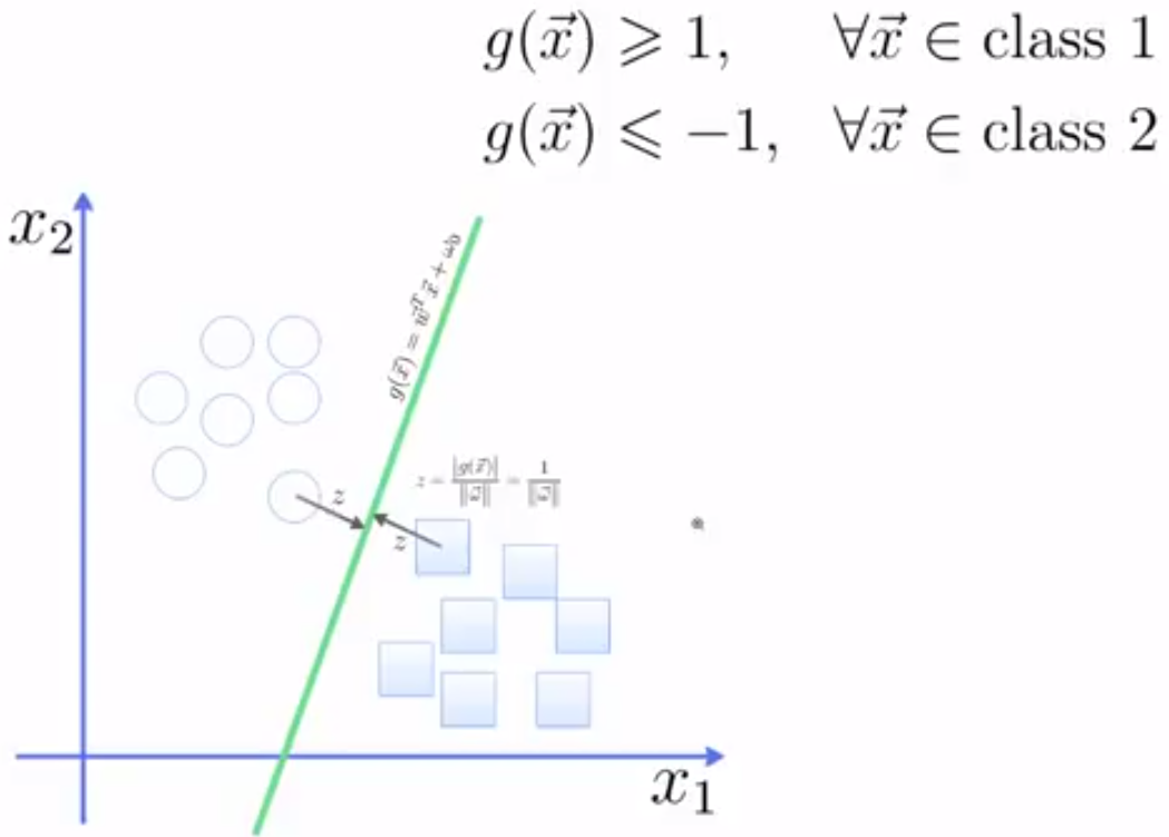
3 支持向量机(线性可分)
假设2维的特征向量, ,有超平面方程: ,所有超平面上方的点满足: ,超平面下方的点满足: ,超平面边际的两边:
简单示例:
from sklearn import svm
x = [[2, 0], [1, 1], [2, 3]] #feature
y = [0, 0, 1]                #label
clf = svm.SVC(kernel = 'linear') #线性核函数
clf.fit(x, y)
print (clf)
# get support vectors
print (clf.support_vectors_)
# get indices of support vectors
print (clf.support_)
# get number of support vectors for each class
print (clf.n_support_)
#predict
print(clf.predict([[2,0]])  )
获得输出:
SVC(C=1.0, cache_size=200, class_weight=None, coef0=0.0,
  decision_function_shape='ovr', degree=3, gamma='auto', kernel='linear',
  max_iter=-1, probability=False, random_state=None, shrinking=True,
  tol=0.001, verbose=False)
[ [1. 1.]
 [2. 3.] ]
[1 2]  #第一、二个点为支持向量(第0个不是)
[1 1]  #在两个类中分别找到几个支持向量
[0]    #预测结果
深入理解:
import numpy as np
import pylab as pl       #画图模块
from sklearn import svm
np.random.seed(0)   #使每次随机生成的值不变
# we create 40 separable points
X = np.r_[np.random.randn(20, 2) - [2, 2], np.random.randn(20, 2) + [2, 2]]
                    #生成20个2维的点,下方,均值和方差都是2;同样20个点,上方。
Y = [0]*20 +[1]*20  #生成标记
#fit the model
clf = svm.SVC(kernel='linear')
clf.fit(X, Y)
# get the separating hyperplane
w = clf.coef_[0]   #coef_存放回归系数,intercept_则存放截距
a = -w[0]/w[1]     #直线斜率
xx = np.linspace(-5, 5)
yy = a*xx - (clf.intercept_[0])/w[1]
# plot the parallels to the separating hyperplane that pass through the support vectors
b = clf.support_vectors_[0]         #第一个支持向量
yy_down = a*xx + (b[1] - a*b[0])    #算出直线
b = clf.support_vectors_[-1]        #另一个支持向量
yy_up = a*xx + (b[1] - a*b[0])      #算出直线
print ("w: ", w);print ("a: ", a)
# print "xx: ", xx;# print "yy: ", yy
print("support_vectors_: ", clf.support_vectors_);print("clf.coef_: ", clf.coef_)
# switching to the generic n-dimensional parameterization of the hyperplan to the 2D-specific equation
# of a line y=a.x +b: the generic w_0x + w_1y +w_3=0 can be rewritten y = -(w_0/w_1) x + (w_3/w_1)
# plot the line, the points, and the nearest vectors to the plane
pl.plot(xx, yy, 'k-')
pl.plot(xx, yy_down, 'k--')
pl.plot(xx, yy_up, 'k--')
#绘制散点图
pl.scatter(clf.support_vectors_[:, 0], clf.support_vectors_[:, 1],s=80, facecolors='none')
pl.scatter(X[:, 0], X[:, 1], c=Y)
pl.axis('tight')
pl.show()
得到如下图所示:
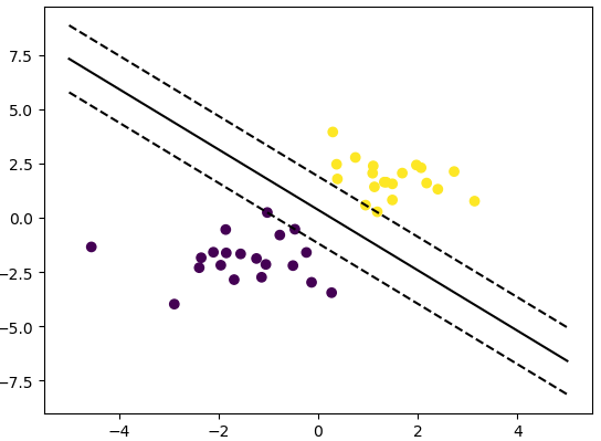
1 训练好的模型的算法复杂度是由支持向量的个数决定的,而不是由数据的维度决定的。所以SVM不太容易产生过拟合;
2 SVM训练出来的模型完全依赖于支持向量,即使训练集里面所有非支持向量的点都被去除,重复训练过程,结果仍然会得到完全一样的模型。
3 如果训练得出的支持向量个数比较小,模型比较容易被泛化。
扫描二维码关注公众号,回复:
2859850 查看本文章

4 支持向量机(线性不可分)
利用一个非线性的映射把原数据集中的向量点转化到一个更高维度的空间中,在这个高维度的空间中找一个线性的超平面来根据线性可分的情况处理。在线性SVM中转化为最优化问题时求解的公式计算都是以内积(dot product)的形式出现,因为内积的算法复杂度非常大,所以利用核函数来取代计算非线性映射函数的内积。。。略。人脸识别示例:
from __future__ import print_function
from time import time
import logging
import matplotlib.pyplot as plt
from sklearn.model_selection import train_test_split
from sklearn.datasets import fetch_lfw_people
from sklearn.model_selection import GridSearchCV
from sklearn.metrics import classification_report
from sklearn.metrics import confusion_matrix
from sklearn.decomposition import PCA
from sklearn.svm import SVC
print(__doc__)
# Display progress logs on stdout
logging.basicConfig(level=logging.INFO, format='%(asctime)s %(message)s')
###############################################################################
# Download the data, if not already on disk and load it as numpy arrays
#下载数据集,wait a moment
lfw_people = fetch_lfw_people(min_faces_per_person=70, resize=0.4)
# introspect the images arrays to find the shapes (for plotting)
n_samples, h, w = lfw_people.images.shape #返回获取数据集的大小(1288,50,37)
# for machine learning we use the 2 data directly (as relative pixel
# positions info is ignored by this model)
X = lfw_people.data #得到数据集特征向量的矩阵,每一行为实例,每一列为特征值
n_features = X.shape[1] #获取特征向量的维度(1表示列),1850,即每个人脸有多少特征
# the label to predict is the id of the person
y = lfw_people.target #获取标记
target_names = lfw_people.target_names #获取人名
n_classes = target_names.shape[0] #对多少个人进行识别
print("Total dataset size:")
print("n_samples: %d" % n_samples) #1288
print("n_features: %d" % n_features) #1850
print("n_classes: %d" % n_classes) #7
###############################################################################
# Split into a training set and a test set using a stratified k fold
# split into a training and testing set,拆分数据集
X_train, X_test, y_train, y_test = train_test_split(X, y, test_size=0.3,random_state=1)
###############################################################################
# Compute a PCA (eigenfaces) on the face dataset (treated as unlabeled,降维
# dataset): unsupervised feature extraction / dimensionality reduction
n_components = 150 #组成元素数量?
print("Extracting the top %d eigenfaces from %d faces"% (n_components, X_train.shape[0]))
t0 = time() #初始化时间
pca = PCA(n_components=n_components, whiten=True).fit(X_train)
print("done in %0.3fs" % (time() - t0))
eigenfaces = pca.components_.reshape((n_components, h, w)) #提取特征
print("Projecting the input data on the eigenfaces orthonormal basis")
t0 = time()
X_train_pca = pca.transform(X_train)
X_test_pca = pca.transform(X_test)
print("done in %0.3fs" % (time() - t0))
###############################################################################
# Train a SVM classification model
print("Fitting the classifier to the training set")
t0 = time()
#设置训练参数:C是惩罚函数,gamma是使用比例,与C结合使用
param_grid = {'C': [1e3, 5e3, 1e4, 5e4, 1e5],'gamma': [0.0001, 0.0005, 0.001, 0.005, 0.01, 0.1], }
#搜索C与gamma中哪一种组合训练的最好
clf = GridSearchCV(SVC(kernel='rbf'), param_grid) #class_weight = 'auto'
clf = clf.fit(X_train_pca, y_train) #建模
print("done in %0.3fs" % (time() - t0))
print("Best estimator found by grid search:")
print(clf.best_estimator_) #最佳估计
###############################################################################
# Quantitative evaluation of the model quality on the test set
print("Predicting people's names on the test set")
t0 = time()
y_pred = clf.predict(X_test_pca) #预测测试集的分类
print("done in %0.3fs" % (time() - t0))
print(classification_report(y_test, y_pred, target_names=target_names)) #将测试集的真实标签与预测的标签相比较
print(confusion_matrix(y_test, y_pred, labels=range(n_classes))) #建立矩阵,对角线上的值越大表示预测准确率越高
###############################################################################
# Qualitative evaluation of the predictions using matplotlib,画图部分,待研究ing
def plot_gallery(images, titles, h, w, n_row=3, n_col=4):
"""Helper function to plot a gallery of portraits"""
plt.figure(figsize=(1.8 * n_col, 2.4 * n_row))
plt.subplots_adjust(bottom=0, left=.01, right=.99, top=.90, hspace=.35)
for i in range(n_row * n_col):
plt.subplot(n_row, n_col, i + 1)
plt.imshow(images[i].reshape((h, w)), cmap=plt.cm.gray)
plt.title(titles[i], size=12)
plt.xticks(())
plt.yticks(())
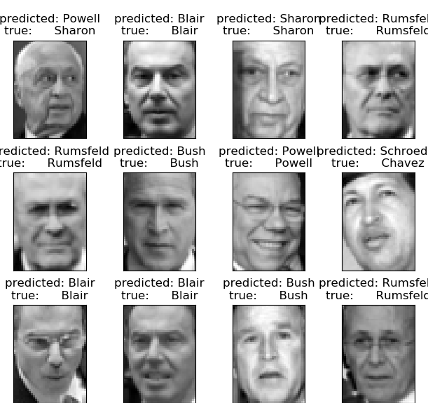
# plot the result of the prediction on a portion of the test set
def title(y_pred, y_test, target_names, i):
pred_name = target_names[y_pred[i]].rsplit(' ', 1)[-1]
true_name = target_names[y_test[i]].rsplit(' ', 1)[-1]
return 'predicted: %s\ntrue: %s' % (pred_name, true_name)
prediction_titles = [title(y_pred, y_test, target_names, i)
for i in range(y_pred.shape[0])]
plot_gallery(X_test, prediction_titles, h, w)
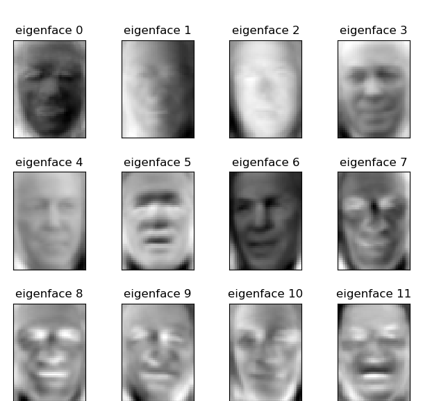
# plot the gallery of the most significative eigenfaces
eigenface_titles = ["eigenface %d" % i for i in range(eigenfaces.shape[0])]
plot_gallery(eigenfaces, eigenface_titles, h, w)
plt.show()输出信息:
None
Total dataset size:
n_samples: 1288
n_features: 1850
n_classes: 7
Extracting the top 150 eigenfaces from 901 faces
done in 0.131s
Projecting the input data on the eigenfaces orthonormal basis
done in 0.021s
Fitting the classifier to the training set
done in 18.547s
Best estimator found by grid search:
SVC(C=1000.0, cache_size=200, class_weight=None, coef0=0.0,
  decision_function_shape='ovr', degree=3, gamma=0.001, kernel='rbf',
  max_iter=-1, probability=False, random_state=None, shrinking=True,
  tol=0.001, verbose=False)
Predicting people's names on the test set
done in 0.054s
                   precision    recall  f1-score   support

     Ariel Sharon       0.67      0.75      0.71        24
     Colin Powell       0.72      0.75      0.73        63
  Donald Rumsfeld       0.74      0.61      0.67        33
    George W Bush       0.88      0.91      0.89       172
Gerhard Schroeder       0.78      0.81      0.79        36
      Hugo Chavez       0.81      0.76      0.79        17
       Tony Blair       0.71      0.64      0.67        42

      avg / total       0.80      0.80      0.80       387

[[ 18   4   2   0   0   0   0]
 [  4  47   1   6   0   2   3]
 [  2   2  20   6   0   0   3]
 [  3   8   2 156   1   1   1]
 [  0   0   1   2  29   0   4]
 [  0   2   0   1   1  13   0]
 [  0   2   1   6   6   0  27]]
输出图像: